Point-wise Discretization Errors in Boundary Element Method for Elasticity Problem
Point-wise Discretization Errors in Boundary Element Method for Elasticity Problem. Bart F. Zalewski Case Western Reserve University Robert L. Mullen Case Western Reserve University. Reliability in Engineering Computing.

Point-wise Discretization Errors in Boundary Element Method for Elasticity Problem
E N D
Presentation Transcript
Point-wise Discretization Errors inBoundary Element Method for Elasticity Problem Bart F. Zalewski Case Western Reserve University Robert L. Mullen Case Western Reserve University
Reliability in EngineeringComputing • For most engineering systems, exact solutions to partial differential equations cannot be obtained. • Numerical methods have been developed to approximate the true solutions by discretizing the governing partial differential equation. • Due to the increase in computing power, many experiments are replaced with numerical simulations. • Thus, there is a growing need for reliability in engineering computing.
Reliability in EngineeringComputing (Cont.) To achieve reliable solutions, the following causes of uncertainty must be addressed: • Uncertainty in the parameters of the system (i.e. material properties) • Uncertainty in boundary conditions • Errors in numerical integration • Errors in solving the resulting linear system of equations • Discretization errors
Why Intervals? • Interval approach is one potential mechanism for handling errors and uncertainties in an integrated and elegant fashion. • Intervals have been used to treat truncation errors, integration errors, and uncertain parameters (p-boxes). • Interval treatment of discretization error for Elasticity problem?
Why Intervals? (Cont.) Interval finite element analysis has been developed to address: • Material, loading, and geometric uncertainty in static problems (Muhanna and Mullen 2001, Neumaier and Pownuk 2007, Modares and Mullen 2008) • Material uncertainty in dynamic problems (Modares and Mullen 2004) • Geometrical instability (Modares et al. 2005)
Why Intervals? (Cont.) Interval boundary element analysis addresses: • Uncertainty in boundary conditions in static problems (Zalewski et al. 2007) • Truncation and integration errors (Zalewski et al. 2007) • Local discretization errors for Laplace equation (Zalewski and Mullen 2007) • Local discretization errors for Elasticity problem (Zalewski and Mullen 2008)
Objective To explore the applications of interval concepts to quantify the discretization error in numerical methods Procedure To use boundary element method as an exemplar of integrated interval treatment of uncertainties and discretization errors
Presentation Outline • Conventional BEA for Elasticity problem (Brebbia 1978) • Local Discretization Error in BEA - Interval Solver - Interval Kernel Splitting Technique - Parametric Interval Solver • Examples • Conclusion
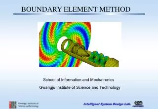
Boundary Element Analysis • Boundary Element Analysis (BEA) is a method for obtaining approximate solutions of partial differential equations. • BEA reduces the dimension of the problem by transforming domain variables to variables on the boundary of the domain using Green’s functions. • The transformed boundary integral equations are solved using collocation methods in which the weighted residual exists only on the boundary of the system. • Source points are located sequentially at all boundary nodes that map domain variables such that they coincide to their nodal values.
Boundary Element Analysisof the Elasticity Problem The Elasticity problem is: is the domain of the system is the boundary of the system , are the values at the boundary
Boundary Element Analysisof the Elasticity Problem (Cont.) The boundary element formulation for the Elasticity problem can be derived starting from Betti’s reciprocal theorem: The equilibrium condition is substituted into the above equation resulting in:
Boundary Element Analysisof the Elasticity Problem (Cont.) The boundary element formulation requires that the weighted residual exists only on the boundary of the domain. This condition is satisfied if the weighted residual function is chosen as the Green’s function which is obtained by applying a concentrated force in direction at a source point as: is the field point at which the response to the concentrated force is measured. The resulting fundamental solution is:
Boundary Element Analysisof the Elasticity Problem (Cont.) and are components of displacement and traction, respectively, due to the applied concentrated force in direction ( j ). These two kernel functions are given as:
Boundary Element Analysisof the Elasticity Problem (Cont.) Substituting the fundamental solution into the integral equation results in: The indices are exchanged in the integral terms and the constant coefficients are cancelled out resulting in: For simplicity the body force is neglected:
Boundary Element Analysisof the Elasticity Problem (Cont.) The boundary integral equation is integrated such that the source point is enclosed by the half-circular boundary of radius , as :
Boundary ElementDiscretization Any boundary can be discretized into boundary elements consisting of nodes, at which a value of either or is known, and assumed polynomial shape functions between nodes. and are vectors of nodal values is a vector of polynomial shape functions
Boundary ElementDiscretization (Cont.) The discretized integral equation is written as: or in matrix form: Applying the boundary conditions, the system of linear equations is rearranged as: and are fully populated non-symmetric matrices and matrix is singular.
Interval Arithmetic In this work errors are treated as interval quantities and interval solutions are shown to guarantee the worst case bounds (interval enclosure) of the true solution.
Interval Arithmetic (Cont.) • The interval number is a closed set as (Moore 1966) and (Neumaier 1990): • Considering two interval numbers: and • Addition: • Subtraction: • Multiplication: • Division: • Subdistributive Property:
Interval Boundary ElementFormulation Interval boundary element analysis treats uncertain boundary conditions, truncation and integration errors (Zalewski et al. 2007): The equation is rearranged as: The system is solved using Newton-Krawczyk iteration (Krawczyk 1969).
Interval Equation Solver The residual Krawczyk iteration is: Substitution:
Interval Equation Solver (Cont.) Regrouping: The iteration follows:
Interval Equation Solver (Cont.) and are mid-point matrices of and
Interval Equation Solver (Cont.) The iteration follows as: If
Discretization Error The boundary is subdivided into elements. For each element, the interval values and are found that bound the functions and over an element such that:
Discretization Error (Cont.) Assuming constant elements results in constant interval bounds on the solution: Assuming linear elements results in linear interval bounds:
Kernel Splitting Technique The kernel splitting technique has been used to bound Fredholm Equations of the First Kind in which the left hand side is deterministic (Dobner 2002). The boundary element integral equations have an interval left hand side and therefore an extended approach is developed.
Interval Kernel Splitting Technique The integral of the product of two functions is bounded as: The right hand side is expressed as a sum of the integrals: or
Interval Kernel SplittingTechnique (Cont.) The interval kernel is of the same sign on , thus can be taken out of the integral on : cannot be taken out of the integral on due to subdistributive property.
Interval Kernel SplittingTechnique (Cont.) The interval kernel is bounded by its limits: where
Interval Kernel SplittingTechnique (Cont.) can be taken out of the integral and the integral equation becomes: The kernels are bounded for all the elements resulting in the system of equations:
Transformation of the Interval Linear System of Equations Considering system of equations: Preconditioning the system: Let , and
Parameterized IntervalEquation Solver • The interval bounds obtained by the solver are not sharp since the dependency of the location of the source point has not been considered. • The uniqueness of the problem is not preserved since two source points are allowed to have the same location at one time resulting in rectangular matrices. • The parameterization considers each source point to have a unique location and allows for sharper interval bounds.
Parameterized IntervalEquation Solver (Cont.) The system is parameterized such that . The system is solved by splitting the kernels for all subintervals such that: This results in the system of equations for each
Parameterized IntervalEquation Solver (Cont.) The system of equations is rearranged: Preconditioning and substitution as described before lead to: The parameterization is incorporated into the solver: is computed when
Parameterized IntervalEquation Solver (Cont.) The difference between the solution and the initial guess is computed and pre-multiplied by the preconditioning matrix : The system is subjected to residual Krawczyk iteration.
Examples The first example obtains the bounds on discretization error for the BEA of the Elasticity problem for the unit square boundary. Boundary Conditions: ubottom=0, tsides=0, uy top=1, tx top=0
Examples (Cont.) The second example shows the behavior of the solution for a hexagonal plate in tension. A symmetry model is considered to decrease computational time.
Conclusions In this work, the point-wise discretization error is bounded using interval methods for the boundary element analysis of the elasticity problem. The examples presented show the capability of the method to enclose the true solution with a desired accuracy. The discretization error is shown to converge with the increasing number of elements, which is the expected behavior. The interval width can be decreased with further parameterization for which the computational cost increases linearly.