What is parametrization? Processes, importance and impact. Testing, validation, diagnostics
350 likes | 514 Views
Introduction to Parametrization of Sub-grid Processes Anton Beljaars (anton.beljaars@ecmwf.int room 114). What is parametrization? Processes, importance and impact. Testing, validation, diagnostics Parametrization development strategy. Why parametrization.

What is parametrization? Processes, importance and impact. Testing, validation, diagnostics
E N D
Presentation Transcript
Introduction to Parametrization of Sub-grid Processes Anton Beljaars(anton.beljaars@ecmwf.int room 114) • What is parametrization? • Processes, importance and impact. • Testing, validation, diagnostics • Parametrization development strategy Introduction to parametrization
Why parametrization • Small scale processes are not resolved by large scale models, because they are sub-grid. • The effect of the sub-grid process on the large scale can only be represented statistically. • The procedure of expressing the effect of sub-grid process is called parametrization. Introduction to parametrization
What is parametrization and why is it needed • The standard Reynolds decomposition and averaging, leads to co-variances that need “closure” or “parametrization” • Radiation absorbed, scattered and emitted by molecules, aerosols and cloud droplets play an important role in the atmosphere and need parametrization. • Cloud microphysical processes need “parametrization” • Parametrization schemes express the effect of sub-grid processes in resolved variables. • Model variables are U,V,T,q, (l,a) Introduction to parametrization
Reynolds decomposition e.g. equation for potential temperature: advection source molecular diffusion Reynolds decomposition: Averaged (e.g. over grid box): : source term (e.g. radiation absorption/emission or condensation) : subgrid (Reynolds) transport term (e.g. due to turbulence, convection) Introduction to parametrization
Space and time scales Introduction to parametrization
Space and time scales 100 hours 1 hour 0.01 hour Introduction to parametrization
Numerical models of the atmosphere Hor. scales Vert. Scales time range • Climate models 500 km 1000 m 100 years • Global weather prediction 50 km 500 m 10 days • Limited area weather pred. 10 km 500 m 2 days • Cloud resolving models 500 m 500 m 1 day • Large eddy models 50 m 50 m 5 hours Different models need different level of parametrization Introduction to parametrization
Parametrized processes in the ECMWF model Introduction to parametrization
Applications and requirements • Applications of the ECMWF model • Data assimilation T799L91-outer and T95L91/T255L91-inner loops: 12-hour 4DVAR. • Medium range forecasts at T799/L91 (25 km): 10 days from 00 and 12 UTC. • Ensemble prediction system at T399L62 (50 km): 10 days, 2x(50+1) members. • Short range at T799L91 (25 km): 3 days, 4 times per day for LAMs. • Seasonal forecasting at T95L40 (200 km): 200 days ensembles coupled to ocean model. • Monthly forecasts (ocean coupled) at T159L61: Every week, 50+1 members. • Fully coupled ocean wave model. • Interim reanalysis (1989-current), under test (possibly T255L91, 4DVAR). • Basic requirements • Accommodate different applications. • Parametrization needs to work over a wide range of spatial resolutions. • Time steps are long (from 15 to 60 minutes); Numerics needs to be efficient and robust. • Interactions between processes are important and should be considered in the design of the schemes. Introduction to parametrization
Importance of physical processes • General • Tendencies from sub-grid processes are substantial and contribute to the evolution of the atmosphere even in the short range. • Diabatic processes drive the general circulation. • Synoptic development • Diabatic heating and friction influence synoptic development. • Weather parameters • Diurnal cycle • Clouds, precipitation, fog • Wind, gusts • T and q at 2m level. • Data assimilation • Forward operators are needed for observations. Introduction to parametrization
Global energy and moisture budgets Energy Moisture 5 mm/day =P-E Hartman, 1994. Academic Press. Fig 6.1 and 5.2 Introduction to parametrization
Sensitivity of cyclo-genesis to surface drag control Pcentre=918 hPa Pcentre=923 hPa analysis Pcentre=925 hPa difference Introduction to parametrization
T-tendencies Introduction to parametrization
T-Tendencies Introduction to parametrization
T-Tendencies Introduction to parametrization
T-Tendencies Introduction to parametrization
T-tendencies Introduction to parametrization
T-Tendencies Imbalance (physics – dynamics) due to: (a) Fast adjustment to initial state (“data assimilation problem”); (b) Parametrization deficiencies Introduction to parametrization
Validation and diagnostics • Compare with analysis • daily verification • systematic errors e.g. from monthly averages • Compare with operational data • SYNOP’s • radio sondes • satellite • Climatological data • ERBE, ISCCP • ocean fluxes • Field experiments • TOGA/COARE, PYREX, ARM, FIFE, ... Introduction to parametrization
Day-5, T850 errors Viterbo and Betts, 1999. JGR, 104D, 27,803-27,810 Introduction to parametrization
History of 2m-T errors over Europe Introduction to parametrization
Surface SW-JJA (model climate - DaSilva climatology) era15 model Introduction to parametrization
PYREX experiment Introduction to parametrization
PYREX mountain drag (Oct/Nov 1990) Lott and Miller, 1995. QJRMS, 121, 1323-1348 Introduction to parametrization
TOGA-COARE fluxes (0-24 h fcsts. vs. ship-observ.) Obs Model era15 model Introduction to parametrization
Cloud fraction (LITE/ECMWF model) Model LITE Introduction to parametrization
Latent heat flux at IMET-buoy Introduction to parametrization
Parametrization development strategy -Invent empirical relations (e.g. based on theory, similarity arguments or physical insight) To find parameters use: • Theory (e.g. radiation) • Field data (e.g. GATE for convection; PYREX for orographic drag; HAPEX for land surface; Kansas for turbulence; ASTEX for clouds; BOREAS for forest albedo) • Cloud resolving models (e.g. for clouds and convection) • Meso scale models (e.g. for subgrid orography) • Large eddy simulation (turbulence) • Test in stand alone or single column mode • Test in 3D mode with short range forecasts • Test in long integrations (model climate) • Consider interactions Introduction to parametrization
Measure diffusion coefficients unstable stable Introduction to parametrization
Convert to empirical function Diffusion coefficients based on Monin Obukhov similarity: MO-scheme (less diffusive) Operational CY30R2 MO-scheme (less diffusive) Operational CY30R2 Introduction to parametrization
Column test Cabauw: July 1987, 3-day time series Observations versus model (T159, 12-36 hr forecasts) Introduction to parametrization
Test in 3D model: Data assimilation + daily forecasts over 32 days March 2004 Effect of MO-stability functions Introduction to parametrization
Concluding remark Enjoy the course and Don’t hesitate to ask questions Introduction to parametrization