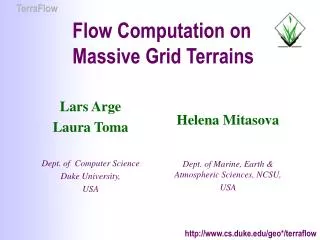
Flow modeling on grid terrains

Flow modeling on grid terrains

Why GIS? • How it all started.. • Duke Environmental researchers: • computing flow accumulation for Appalachian Mountains took 14 days (with 512MB memory) • 800km x 800km at 100m resolution  ~64 million points • GIS (Geographic Information Systems) • System that handles spatial data • Visualization, processing, queries, analysis… • Rich area of problems for Computer Science • Graphics, graph theory, computational geometry, scientific computing…

Indispensable tool Monitoring:keep an eye on the state of earth systems using satellites and monitoring stations (water, pollution, ecosystems, urban development,…) Modeling and simulation: predict consequences of human actions and natural processes Analysis and risk assessment:find the problem areas and analyse the possible causes (soil erosion, groundwater pollution,..) Planning and decision support: provide information and tools for better management of resources Precipitation in Tropical South America Lots of rain Dry Nitrogen in Chesapeake Bay High nitrogen concentrations GIS and the Environment

GIS and the Environment Bald Head Island Renourishment Sediment flow

3 3 3 3 2 2 2 2 4 4 4 4 7 7 7 7 5 5 5 5 8 8 8 8 7 7 7 7 1 1 1 1 9 9 9 9 DEM Representations TIN Grid Contour lines Sample points

Reality: Elevation of terrain is a continuous function of two variables h(x,y) Estimate, predict, simulate Flooding, pollution Erosion, deposition Vegetation structure …. GIS: DEM (Digital Elevation Model) is a set of sample points and their heights { x, y, hxy} Computations on Terrains Model and compute indices

Modeling Flow on Terrains • What happens when it rains? • Predict areas susceptible to floods. • Predict location of streams. • Compute watersheds. • Flow is modeled using two basic attributes • Flow Direction (FD) • The direction water flows at a point • Flow Accumulation (FA) • Total amount of water that flows through a point (if water is distributed according to the flow directions)

Flow Direction (FD) on Grids • Water flows downhill • follows the gradient • On grids: Approximated using 3x3 neighborhood • SFD (Single-Flow Direction): • FD points to the steepest downslope neighbor • MFD (Multiple-Flow direction) : • FD points to all downslope neighbors

Computing FD • Goal: compute FD for every cell in the grid (FD grid) • Algorithm: • Scan the grid • For each cell compute SFD/MFD by inspecting 8 neighbor cells • Analysis: O(N) time for a grid of N cells • Is this all? • NO! flat areas: Plateas and sinks

FD on Flat Areas • …no obvious flow direction • Plateaus • Assign flow directions such that each cell flows towards the nearest spill point of the plateau • Sinks • Either catch the water inside the sink • Or route the water outside the sink using uphill flow directions • model steady state of water and remove (fill) sinks by simulating flooding: uniformly pouring water on terrain until steady state is reached • Assign uphill flow directions on the original terrain by assigning downhill flow directions on the flooded terrain

Flow Accumulation (FA) on Grids FA models water flow through each cell with “uniform rain” • Initially one unit of water in each cell • Water distributed from each cell to neighbors pointed to by its FD • Flow conservation: If several FD, distribute proportionally to height difference • Flow accumulation of cell is total flow through it Goal: compute FA for every cell in the grid (FA grid)

Computing FA • FD graph: • node for each cell • (directed) edge from cell a to b if FD of a points to b • FD graph must be acyclic • ok on slopes, be careful on plateaus • FD graph depends on the FD method used • SFD graph: a tree (or a set of trees) • MFD graph: a DAG (or a set of DAGs)

Computing FA: Plane Sweeping • Input: flow direction grid FD • Output: flow accumulation grid FA (initialized to 1) • Process cells in topological order. For each cell: • Read its flow from FA grid and its direction from FD grid • Update flow for downslope neighbors (all neighbors pointed to by cell flow direction) • Correctness • One sweep enough • Analysis • O(sort) + O(N) time for a grid of N cells • Note: Topological order means decreasing height order (since water flows downhill).

DEM and Flow Accumulation[Panama]

Flow accumulation with MFD

Flow accumulation with SFD

Uses Flow direction and flow accumulation are used for: • Computing other hydrological attributes • river network • moisture indices • watersheds and watershed divides • Analysis and prediction of sediment and pollutant movement in landscapes. • Decision support in land management, flood and pollution prevention and disaster management

Remote sensing technology Massive amounts of terrain data Higher resolutions (1km, 100m, 30m, 10m, 1m,…) NASA-SRTM Mission launched in 2001 Acquired data for 80% of earth at 30m resolution 5TB USGS Most of US at 10m resolution LIDAR 1m res Massive Terrain Data

Example: LIDAR Terrain Data • Massive (irregular) point sets (1-10m resolution) • Relatively cheap and easy to collect Example: Jockey’s ridge (NC coast)

It’s Growing! • Appalachian Mountains Area if approx. 800 km x 800 km Sampled at: • 100m resolution:  64 million points (128MB) • 30m resolution:  640 (1.2GB) • 10m resolution:  6400 = 6.4 billion (12GB) • 1m resolution:  600.4 billion (1.2TB)

Computing on Massive Data • GRASS (open source GIS) • Killed after running for 17 days on a 6700 x 4300 grid (approx 50 MB dataset) • TARDEM (research, U. Utah) • Killed after running for 20 days on a 12000 x 10000 grid (appox 240MB dataset) • CPU utilization5%, 3GB swap file • ArcInfo (ESRI, commercial GIS) • Can handle the 240MB dataset • Doesn’t work for datasets bigger than 2GB

Dataset Size (log) Scalability Problem • We can compute FD and FA using simple O(N)-time algorithms • ..but.. for large sets..??

read/write head read/write arm track magnetic surface Scalability Problem: Why? • Most (GIS) programs assume data fits in memory • minimize only CPU computation • But.. Massive data does not fit in main memory! • OS places data on disk and moves data between memory and disk as needed • Disk systems try to amortize large access time by transferring large contiguous blocks of data • When processing massive data disk I/O is the bottleneck, rather than CPU time!

Disks are Slow “The difference in speed between modern CPU and disk technologies is analogous to the difference in speed in sharpening a pencil using a sharpener on one’s desk or by taking an airplane to the other side of the world and using a sharpener on someone else’s desk.” (D. Comer)

Scalability to Large Data • Example: reading an array from disk • Array size N = 10 elements • Disk block size = 2 elements • Memory size = 4 elements (2 blocks) 1 5 2 6 3 8 9 4 7 10 1 2 10 9 5 6 3 4 8 7 Algorithm 1: Loads 10 blocks Algorithm 2: Loads 5 blocks N blocks >> N/B blocks • Block size is large (32KB, 64KB) N >> N/B N = 256 x 106, B = 8000 , 1ms disk access time  NI/Os take 256 x 103 sec = 4266 min = 71 hr  N/BI/Os take 256/8 sec = 32 sec

I/O-model I/O-operation Read/write one block of data from/to disk I/O-complexity number of I/O-operations (I/Os) performed by the algorithm External memory or I/O-efficient algorithms: Minimize I/O-complexity • RAM model • CPU-operation • CPU-complexity • Number of CPU-operations performed by the algorithm • Internal memory algorithms: • Minimize CPU-complexity

I/O-Model D Parameters N = # elements in problem instance B = # elements that fit in disk block M = # elements that fit in main memory Fundamental bounds: • Scanning: scan(N) = • Sorting: sort(N) = Block I/O M P In practiceblock and main memory sizes are big

TerraFlow • TerraFlow is our suite of programs for flow routing and flow accumulation on massive grids[ATV`00,AC&al`02] • Flow routing and flow accumulation modeled as graph problems and solved in optimal I/O bounds • Efficient • 2-1000 times faster on very large grids than existing software • Scalable • 1 billion elements!! (>2GB data) • Flexible • Allows multiple methods flow modeling http://www.cs.duke.edu/geo*/terraflow

TerraFlow • GRASS cannot handle Hawaii dataset (killed after 17 days) • TARDEM cannot handle Cumberlands dataset (killed after 20 days) • Significant speedup over ArcInfo for large datasets • East-Coast TerraFlow: 8.7 Hours ArcInfo: 78 Hours • Washington state TerraFlow: 63 Hours ArcInfo: %

Massive Data • Massive datasets are being collected everywhere • Storage management software is billion-$ industry (More) Examples: • Phone: AT&T 20TB phone call database, wireless tracking • Consumer: WalMart 70TB database, buying patterns (supermarket checkout) • WEB: Web crawl of 200M pages and 2000M links, Akamai stores 7 billion clicks per day • Geography: NASA satellites generate 1.2TB per day

Flow modeling on grid terrains