Download
1 / 30
300 likes | 445 Views
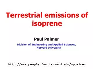
Terrestrial and marine emissions of isoprene. Paul Palmer Division of Engineering and Applied Sciences, Harvard University. http://www.people.fas.harvard.edu/~ppalmer. hv. O 3. NO 2. NO. OH. HO 2. HC+OH HCHO + products. NOx, HC, CO.

E N D
Terrestrial and marine emissions of isoprene Paul Palmer Division of Engineering and Applied Sciences, Harvard University http://www.people.fas.harvard.edu/~ppalmer
hv O3 NO2 NO OH HO2 HC+OH HCHO + products NOx, HC, CO Tropospheric O3 is an important climate forcing agent Level of Scientific Understanding Natural VOC emissions (50% isoprene) ~ CH4 emissions. IPCC, 2001
GEIA EPA BEIS2 7.1 Tg C 2.6 Tg C MEGAN [1012 atom C cm-2 s-1] 3.6 Tg C Isoprene emissions July 1996 Isoprene oxidation products (e.g. HCHO) provide constraints on estimated emissions
GOME isoprene emissions (July 1996) agree with surface measurements ppb 0 12 r2 = 0.53 Bias -3% r2 = 0.65 Bias -30% BEIS2 GEIA Modeled HCHO [ppb] Observed HCHO [ppb]
LAI Sep April Modeling the terrestrial biosphere PAR – direct and diffuse (GMAO) Temperature: Instantaneous (G95) 10-day avg (Petron ‘01) Fixed base emission factors (Guenther 2004) Canopy model (Guenther 1995) Altitude Emission MODIS/AVHRR LAI Emissions
GEOS-CHEM Global 3D CTM PAR, T Emissions MODEL BIOSPHERE MEGAN (isoprene) Canopy model Leaf age LAI Temperature Base factors GEIA Monoterpenes MBO Acetone Methanol Global 3-D Modeling Overview • Driven by NASA GMAO met data • 2x2.5o resolution/30 vertical levels • O3-NOx-VOC-aerosol chemistry Monthly mean LAI (AVHRR/MODIS)
Monoterpenes Isoprene MBO May Jun Jul Aug Sep VOC emissions during 2001 growing season [1012 atom C cm-2 s-1]
NOx = 1 ppb NOx = 0.1 ppb 0.4 pinene ( pinene similar) DAYS HCHO production from biogenics using the MCM Y become closer at t progresses further isoprene 0.5 0.33 Cumulative HCHO yield [per C] GEOS-CHEM HOURS Use this analysis to parameterise source of HCHO from monoterpenes Mike Pilling and Jenny Stanton, Leeds University
Global Ozone Monitoring Experiment • Nadir-viewing SBUV instrument • Pixel 320 x 40 km2 • 10.30 am cross-equator time (globe in 3 days) • O3, NO2, BrO, OClO, SO2, HCHO, H2O, cloud • HCHO slant columns fitted: 337-356nm • Fitting uncertainty < continental signals Isoprene Biomass Burning HCHO JULY 1997
GEOS-CHEM GEOS-CHEM GOME GOME May Aug Jun Sep Jul GROWING SEASON 2001 HCHO column [1016 molec cm-2] HCHO column signal from monoterpenes is comparable to GOME column uncertainty
HCHO data over the Ozarks SOS 1999 Aircraft data @ 350 m July 1999 Illinois Missouri Kansas OZARKS [ppb] GOME c/o Y-N. Lee, Brookhaven National Lab. [1016 molec cm-2]
kHCHOHCHO EVOC = _______________ kVOCYieldVOCHCHO hours WHCHO hours Isoprene HCHO h, OH OH a-pinene propane VOC 100 km Distance downwind VOC source Relating HCHO Columns to VOC Emissions Master Chemical Mechanism
Wind direction associated with largest [HCHO] in 1998 intensive EVALUATE GOME DATA USING LONG-TERM ISOPRENE FLUX DATA PROPHET RESEARCH SITE (MI) Maple, beech, birch, basswood, mixed aspen, bog conifers (lower, wet areas), and pine and red oak (drier upland regions). Average height near 20 m. Overstory age of the hardwood forest is approximately 75 years.
Isoprene flux [1012 molec cm-2 s-1] Measured (WSU) MEGAN GOME Using observed isop flux:HCHO column regression better agreement with GOME Long term in situ isoprene flux measurements at PROPHET site during 2001 Isoprene flux [1012 molec cm-2 s-1] Measured (WSU) MEGAN GOME HCHO column [1016 molec cm-2] +/- uncertainty Y2K1 Day
May July June September August 1996 1997 1998 1999 2000 2001 HCHO column [1016 molec cm-2]
Interannual variability of the seasonal cycle GOME HCHO Column [1016 molec cm-2] Southeast US 32-38N; 265-280W Days 2K1
GOME HCHO Column [1016 molec cm-2] r = 0.75 n=14 PAMS (EPA) Isoprene Concentration (10-12 LT) [ppbC] In situ observations over Atlanta GA provide some verification of large interannual variability Mean values associated with individual values > 30 ppbC Lance McCluney, EPA
What is driving this variability? 2nd-order polynomial fit to HCHO columns Curve based on greenhouse data (Guenther) r=0.9
Terrestrial Biosphere: Remarks • GOME HCHO data provide constraints on natural VOC emissions • Data consistent with seasonal and interannual variability observed with in situ measurements • Improved understanding and quantification of air quality and climate • Just the beginning…need to relate model-observation discrepancy to a better understanding of the underlying processes
Marine Biosphere Isoprene Prochlorococcus Photo by Claire Ting 0.7m Emiliania huxleyi Photo by Jeremy Young Micromonas pusilla Mats Kuylenstierna & Bengt Karlson • Phytoplankton responsible for 50% of global photosynthesis and oxygen production • Other organisms also important, e.g. seaweed
Emissions from the marine biosphere – a coupling between biology, chemistry and physics Dynamics VOCs, oxygenates, DMS UVB Isoprene Phytoplankton Depth [m] Chlorophyll Bacteria Nutrients Viruses
Measured relationship between isoprene production and chlorophyll using laboratory culture Production ~invariant with cell volume Phytoplankton studied in size order: Prochlorococcus (n=8), Synechococcus (n=2), M. Pusilla (n=1), P. Calceolata (n=1), E. Huxleyi (n=2) Shaw et al, 2003
Terra MODIS (MODerate Resolution Imaging Spectrometer) • Polar sun-synchronous orbit 10.30AM descending mode. Earth surface within a few days. • Measures 36 discrete spectral bands with a 2,330 km wide swath. • Chlorophyll-a content retrieval algorithm fits absorption coefficient @ 675nm (phytoplankton) and absorption @ 400nm (coloured DOM) • Uncertainty ~30%
1x10⁻⁴ 1x10⁻⁴ 1x10⁻² 1x10⁻² 1x10⁻⁶ 1x10⁻⁶ January 2001 Scaling of MODIS chlorophyll-a observations global isoprene ocean production rates [molec cm-2 s-1] July 2001
Sinks of isoprene in seawater Air-sea exchange Ventilation of ocean mixed layerO(3-4 days) Chemical 1O2: [1O2]=10-13 M; k(1O2)=106 1/Msec = 115 days OH: [OH]=610 M; k(OH)=10-17 = 19 days Biological Loss O(15-20 days)Dynamics Mixing down to deeper ocean: > air-sea exchange Advection (not sink on regional scale): O(10 days) Assume Isoprene is in SS: P – L =0
Air-sea flux F = K ( CW – CA/H) K = gas exchange coefficient (piston velocity) = 0.31 U2 (Sc/660)-0.5 ; Wind Speed U from QuikScat Sc = Schmidt number (SST dependent); T from MODIS = kinematic viscocity/diffusion coefficient CW = seawater concentration CA = atmospheric concentration = 0 for isoprene over ocean! H =Henry’s law constant
January 2001 Validation with sparse in situ data 7.4x10⁸ E. Atlantic NW. Pacific MODIS Isoprene Flux [molec cm-2 s-1] Florida Straits In situ Isoprene Flux [molec cm-2 s-1] Global Isoprene Fluxes Estimated from MODIS July 2001 4.6x10⁸
DJF MAMJJASON Isoprene flux [108 molec cm-2 s-1] Latitude [deg] Seasonal fluxes of isoprene from the marine biosphere Rise and fall consistent with phytoplankton blooms
Marine Biosphere Isoprene Flux [Tg/month] Annual budget 0.2 Tg/yr 2K1 Month Global Isoprene Budgets Global budgets estimated from in situ data (Tg/yr) 1.2 Bonsang et al, 1992 0.4 Milne et al, 1995 Terrestrial biosphere ~400 Tg/yr Marine biosphere fluxes 0.8 ppt isoprene Terrestrial biosphere fluxes 0.4 ppb isoprene
Closing Remarks • MODIS isoprene fluxes are largely consistent with in situ flux measurements • Global marine isoprene flux is small compared with terrestrial source – regional importance? • Methodology can be applied to more climatically important trace gases – seawater chemistry more complicated • Both studies show clearly the utility of satellite observations to better understand the biosphere • Also need to appreciate the importance of in situ measurements