Download
1 / 46
460 likes | 689 Views
Biological Motif Discovery. Concepts Motif Modeling and Motif Information EM and Gibbs Sampling Comparative Motif Prediction Applications Transcription Factor Binding Site Prediction Epitope Prediction Lab Practical DNA Motif Discovery with MEME and AlignAce

E N D
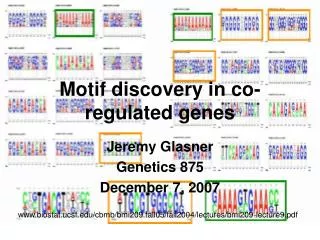
Biological Motif Discovery Concepts Motif Modeling and Motif Information EM and Gibbs Sampling Comparative Motif Prediction Applications Transcription Factor Binding Site Prediction Epitope Prediction Lab Practical DNA Motif Discovery with MEME and AlignAce Co-regulated genes from TB Boshoff data set
Regulatory Motifs Find promoter motifs associated with co-regulated or functionally related genes
Transcription Factor Binding Sites • Very Small • Highly Variable • ~Constant Size • Often repeated • Low-complexity-ish Slide Credit: S. Batzoglou
Other “Motifs” • Splicing Signals • Splice junctions • Exonic Splicing Enhancers (ESE) • Exonic Splicing Surpressors (ESS) • Protein Domains • Glycosylation sites • Kinase targets • Targetting signals • Protein Epitopes • MHC binding specificities
Essential Tasks • Modeling Motifs • How to computationally represent motifs • Visualizing Motifs • Motif “Information” • Predicting Motif Instances • Using the model to classify new sequences • Learning Motif Structure • Finding new motifs, assessing their quality
Consensus Sequences Useful for publication IUPAC symbols for degenerate sites Not very amenable to computation Nature Biotechnology 24, 423 - 425 (2006)
Count frequencies Add pseudocounts 1 K Probabilistic Model M1 MK M1 A C G T .1 .2 .1 .4 .1 .1 .2 .2 .2 .2 .5 .1 .4 .5 .4 .2 .2 .1 .3 .1 .2 .2 .2 .7 Pk(S|M) Position Frequency Matrix (PFM)
A C G T A C G T .1 .2 .1 .4 .1 .1 -1.3 -0.3 -1.3 0.6 -1.3 -1.3 .2 .2 .2 .2 .5 .1 -0.3 -0.3 0.3 -0.3 1 -1.3 .4 .5 .4 .2 .2 .1 0.6 1 0.6 -0.3 -0.3 -1.3 .3 .1 .2 .2 .2 .7 0.3 -1.3 -0.3 -0.3 -0.3 1.4 Scoring A Sequence To score a sequence, we compare to a null model Log likelihood ratio Position Weight Matrix (PWM) Background DNA (B) PFM
Scoring a Sequence Common threshold = 60% of maximum score MacIsaac & Fraenkel (2006) PLoS Comp Bio
Visualizing Motifs – Motif Logos Represent both base frequency and conservation at each position Height of letter proportional to frequency of base at that position Height of stack proportional to conservation at that position
Motif Information The height of a stack is often called the motif information at that position measured in bits Information Why is this a measure of information?
Average Uncertainty Two possible outcomes for sun rising A “The sun will rise tomorrow” P(A)=p1 B “The sun will not rise tomorrow” P(B)=p2 What is our average uncertainty about the sun rising = Entropy
Entropy Entropy measures average uncertainty Entropy measures randomness If log is base 2, then the units are called bits
1 0.9 0.8 0.7 0.6 0.5 0.4 0.3 0.2 0.1 0 0 0.1 0.2 0.3 0.4 0.5 0.6 0.7 0.8 0.9 1 Entropy versus randomness Entropy is maximum at maximum randomness Example: Coin Toss P(heads)=0.1 Not very random H(X)=0.47 bits Entropy P(heads)=0.5 Completely random H(X)=1 bits P(heads)
1 0.9 0.8 0.7 0.6 P(x) 0.5 0.4 0.3 0.2 0.1 0 A 1 A 1 2 T 2 T 3 G 3 G C 4 4 C 1 0.9 0.8 0.7 0.6 P(x) 0.5 0.4 0.3 0.2 0.1 0 Entropy Examples
Information Content Information is a decrease in uncertainty Once I tell you the sun will rise, your uncertainty about the event decreases Information = Hbefore(X) - Hafter(X) Information is difference in entropy after receiving information
1 1 0.9 0.9 0.8 0.8 0.7 0.7 0.6 0.6 0.5 0.5 0.4 0.4 0.3 0.3 0.2 0.2 0.1 0.1 0 0 A A T T G G C C Motif Information 2 - Motif Position Information = Hbackground(X) Hmotif_i(X) Uncertainty after learning it is position i in a motif Prior uncertainty about nucleotide P(x) P(x) H(X)=2 bits H(X)=0.63 bits Uncertainty at this position has been reduced by 0.37 bits
Motif Logo Conserved Residue Reduction of uncertainty of 2 bits Little Conservation Minimal reduction of uncertainty
1 1 0.9 0.9 0.8 0.8 0.7 0.7 0.6 0.6 0.5 0.5 0.4 0.4 (e.g. Plasmodium) 0.3 0.3 Hmotif_i(X) Hbackground(X) 0.2 0.2 0.1 0.1 0 0 A A T T G G C C P(x) P(x) H(X)=1.7 bits H(X)=1.9 bits 1.7 Background DNA Frequency The definition of information assumes a uniform background DNA nucleotide frequency What if the background frequency is not uniform? 2 - Motif Position Information = = -0.2 bits Some motifs could have negative information!
A Different Measure Relative entropy or Kullback-Leibler (KL) divergence Divergence between a “true” distribution and another “True” Distribution Other Distribution Properties DKL is larger the more different Pmotif is from Pbackground Same as Information if Pbackground is uniform
Comparing Both Methods Information assuming uniform background DNA KL Distance assuming 20% GC content (e.g. Plasmodium)
Online Logo Generation http://weblogo.berkeley.edu/ http://biodev.hgen.pitt.edu/cgi-bin/enologos/enologos.cgi
Finding New Motifs Learning Motif Models
Background DNA M1 MK M1 A C G T .1 .2 .1 .4 .1 .3 .2 .2 .2 .2 .5 .4 .4 .5 .4 .2 .2 .2 .3 .1 .2 .2 .2 .1 P(S|B) A Promoter Model Length K Motif Pk(S|M) The same motif model in all promoters
.1 .2 .1 .4 .1 .3 .2 .2 .2 .2 .5 .4 M1 MK M1 .4 .5 .4 .2 .2 .2 Si = nucleotide at position i in the sequence .3 .1 .2 .2 .2 .1 A C G T Probability of a Sequence Given a sequence(s), motif model and motif location 1 60 65 100 A T A T G C
M1 M1 M6 A C G T 3/4 ETC… 3/4 Parameterizing the Motif Model Given multiple sequences and motif locations but no motif model AATGCG ATATGG ATATCG GATGCA Count Frequencies Add pseudocounts
x x x x Finding Known Motifs Given multiple sequences and motif model but no motif locations P(Seqwindow|Motif) window Calculate P(Seqwindow|Motif) for every starting location Choose best starting location in each sequence
Discovering Motifs Given a set of co-regulated genes, we need to discover with only sequences We have neither a motif model nor motif locations Need to discover both How can we approach this problem? (Hint: start with a random motif model)
Expectation Maximization (EM) • Remember the basic idea! • Use model to estimate (distribution of) missing data • Use estimate to update model • Repeat until convergence Model is the motif model Missing data are the motif locations
A C G T A C G T .1 .1 .2 .1 .1 .1 .1 .4 .1 .1 .3 .3 .2 .2 .3 .2 .2 .2 .2 .2 .5 .5 .4 .1 .4 .4 .5 .5 .4 .4 .5 .2 .2 .2 .1 .2 .3 .3 .1 .1 .2 .2 .2 .2 .2 .2 .1 .1 EM for Motif Discovery • Start with random motif model • E Step: estimate probability of motif positions for each sequence • M Step: use estimate to update motif model • Iterate (to convergence) At each iteration, P(Sequences|Model) guaranteed to increase ETC…
MEME • MEME - implements EM for motif discovery in DNA and proteins • MAST – search sequences for motifs given a model http://meme.sdsc.edu/meme/
EM starts at an initial set of parameters And then “climbs uphill” until it reaches a local maximum P(Seq|Model) Landscape EM searches for parameters to increase P(seqs|parameters) Useful to think of P(seqs|parameters) as a function of parameters P(Sequences|params1,params2) Parameter1 Parameter2 Where EM starts can make a big difference
Search from Many Different Starts To minimize the effects of local maxima, you should search multiple times from different starting points MEME uses this idea Start at many points Run for one iteration Choose starting point that got the “highest” and continue P(Sequences|params1,params2) Parameter1 Parameter2
Gibbs Sampling A stochastic version of EM that differs from deterministic EM in two key ways • At each iteration, we only update the motif position • of a single sequence • 2. We may update a motif position to a “suboptimal” new position
A C G T A C G T .1 .1 .2 .1 .1 .1 .1 .4 .1 .1 .3 .3 .2 .2 .2 .3 .2 .2 .2 .2 .5 .5 .1 .4 .4 .4 .5 .5 .4 .4 .2 .5 .2 .2 .2 .1 .3 .3 .1 .1 .2 .2 .2 .2 .2 .2 .1 .1 Gibbs Sampling • Start with random motif locations and calculate a motif model • Randomly select a sequence, remove its motif and recalculate tempory model • With temporary model, calculate probability of motif at each position on sequence • Select new position based on this distribution • Update model and Iterate “Best” Location New Location ETC…
Gibbs Sampling and Climbing Because gibbs sampling does not always choose the best new location it can move to another place not directly uphill P(Sequences|params1,params2) Parameter1 Parameter2 In theory, Gibbs Sampling less likely to get stuck a local maxima
AlignACE • Implements Gibbs sampling for motif discovery • Several enhancements • ScanAce – look for motifs in a sequence given a model • CompareAce – calculate “similarity” between two motifs (i.e. for clustering motifs) http://atlas.med.harvard.edu/cgi-bin/alignace.pl
Assessing Motif Quality Scan the genome for all instances and associate with nearest genes • Category Enrichment – look for association between motif and sets of genes. Score using Hypergeometric distribution • Functional Category • Gene Families • Protein Complexes • Group Specificity – how restricted are motif instances to the promoter sequences used to find the motif? • Positional Bias – do motif instances cluster at a certain distance from ATG? • Orientation Bias– do motifs appear preferentially upstream or downstream of genes?
TBP GAL4 GAL4 GAL4 GAL4 MIG1 MIG1 TBP Factor footprint Conservation island Conservation of Motifs GAL10 Scer TTATATTGAATTTTCAAAAATTCTTACTTTTTTTTTGGATGGACGCAAAGAAGTTTAATAATCATATTACATGGCATTACCACCATATACA Spar CTATGTTGATCTTTTCAGAATTTTT-CACTATATTAAGATGGGTGCAAAGAAGTGTGATTATTATATTACATCGCTTTCCTATCATACACA Smik GTATATTGAATTTTTCAGTTTTTTTTCACTATCTTCAAGGTTATGTAAAAAA-TGTCAAGATAATATTACATTTCGTTACTATCATACACA Sbay TTTTTTTGATTTCTTTAGTTTTCTTTCTTTAACTTCAAAATTATAAAAGAAAGTGTAGTCACATCATGCTATCT-GTCACTATCACATATA * * **** * * * ** ** * * ** ** ** * * * ** ** * * * ** * * * Scer TATCCATATCTAATCTTACTTATATGTTGT-GGAAAT-GTAAAGAGCCCCATTATCTTAGCCTAAAAAAACC--TTCTCTTTGGAACTTTCAGTAATACG Spar TATCCATATCTAGTCTTACTTATATGTTGT-GAGAGT-GTTGATAACCCCAGTATCTTAACCCAAGAAAGCC--TT-TCTATGAAACTTGAACTG-TACG Smik TACCGATGTCTAGTCTTACTTATATGTTAC-GGGAATTGTTGGTAATCCCAGTCTCCCAGATCAAAAAAGGT--CTTTCTATGGAGCTTTG-CTA-TATG Sbay TAGATATTTCTGATCTTTCTTATATATTATAGAGAGATGCCAATAAACGTGCTACCTCGAACAAAAGAAGGGGATTTTCTGTAGGGCTTTCCCTATTTTG ** ** *** **** ******* ** * * * * * * * ** ** * *** * *** * * * Scer CTTAACTGCTCATTGC-----TATATTGAAGTACGGATTAGAAGCCGCCGAGCGGGCGACAGCCCTCCGACGGAAGACTCTCCTCCGTGCGTCCTCGTCT Spar CTAAACTGCTCATTGC-----AATATTGAAGTACGGATCAGAAGCCGCCGAGCGGACGACAGCCCTCCGACGGAATATTCCCCTCCGTGCGTCGCCGTCT Smik TTTAGCTGTTCAAG--------ATATTGAAATACGGATGAGAAGCCGCCGAACGGACGACAATTCCCCGACGGAACATTCTCCTCCGCGCGGCGTCCTCT Sbay TCTTATTGTCCATTACTTCGCAATGTTGAAATACGGATCAGAAGCTGCCGACCGGATGACAGTACTCCGGCGGAAAACTGTCCTCCGTGCGAAGTCGTCT ** ** ** ***** ******* ****** ***** *** **** * *** ***** * * ****** *** * *** Scer TCACCGG-TCGCGTTCCTGAAACGCAGATGTGCCTCGCGCCGCACTGCTCCGAACAATAAAGATTCTACAA-----TACTAGCTTTT--ATGGTTATGAA Spar TCGTCGGGTTGTGTCCCTTAA-CATCGATGTACCTCGCGCCGCCCTGCTCCGAACAATAAGGATTCTACAAGAAA-TACTTGTTTTTTTATGGTTATGAC Smik ACGTTGG-TCGCGTCCCTGAA-CATAGGTACGGCTCGCACCACCGTGGTCCGAACTATAATACTGGCATAAAGAGGTACTAATTTCT--ACGGTGATGCC Sbay GTG-CGGATCACGTCCCTGAT-TACTGAAGCGTCTCGCCCCGCCATACCCCGAACAATGCAAATGCAAGAACAAA-TGCCTGTAGTG--GCAGTTATGGT ** * ** *** * * ***** ** * * ****** ** * * ** * * ** *** Scer GAGGA-AAAATTGGCAGTAA----CCTGGCCCCACAAACCTT-CAAATTAACGAATCAAATTAACAACCATA-GGATGATAATGCGA------TTAG--T Spar AGGAACAAAATAAGCAGCCC----ACTGACCCCATATACCTTTCAAACTATTGAATCAAATTGGCCAGCATA-TGGTAATAGTACAG------TTAG--G Smik CAACGCAAAATAAACAGTCC----CCCGGCCCCACATACCTT-CAAATCGATGCGTAAAACTGGCTAGCATA-GAATTTTGGTAGCAA-AATATTAG--G Sbay GAACGTGAAATGACAATTCCTTGCCCCT-CCCCAATATACTTTGTTCCGTGTACAGCACACTGGATAGAACAATGATGGGGTTGCGGTCAAGCCTACTCG **** * * ***** *** * * * * * * * * ** Scer TTTTTAGCCTTATTTCTGGGGTAATTAATCAGCGAAGCG--ATGATTTTT-GATCTATTAACAGATATATAAATGGAAAAGCTGCATAACCAC-----TT Spar GTTTT--TCTTATTCCTGAGACAATTCATCCGCAAAAAATAATGGTTTTT-GGTCTATTAGCAAACATATAAATGCAAAAGTTGCATAGCCAC-----TT Smik TTCTCA--CCTTTCTCTGTGATAATTCATCACCGAAATG--ATGGTTTA--GGACTATTAGCAAACATATAAATGCAAAAGTCGCAGAGATCA-----AT Sbay TTTTCCGTTTTACTTCTGTAGTGGCTCAT--GCAGAAAGTAATGGTTTTCTGTTCCTTTTGCAAACATATAAATATGAAAGTAAGATCGCCTCAATTGTA * * * *** * ** * * *** *** * * ** ** * ******** **** * Scer TAACTAATACTTTCAACATTTTCAGT--TTGTATTACTT-CTTATTCAAAT----GTCATAAAAGTATCAACA-AAAAATTGTTAATATACCTCTATACT Spar TAAATAC-ATTTGCTCCTCCAAGATT--TTTAATTTCGT-TTTGTTTTATT----GTCATGGAAATATTAACA-ACAAGTAGTTAATATACATCTATACT Smik TCATTCC-ATTCGAACCTTTGAGACTAATTATATTTAGTACTAGTTTTCTTTGGAGTTATAGAAATACCAAAA-AAAAATAGTCAGTATCTATACATACA Sbay TAGTTTTTCTTTATTCCGTTTGTACTTCTTAGATTTGTTATTTCCGGTTTTACTTTGTCTCCAATTATCAAAACATCAATAACAAGTATTCAACATTTGT * * * * * * ** *** * * * * ** ** ** * * * * * *** * Scer TTAA-CGTCAAGGA---GAAAAAACTATA Spar TTAT-CGTCAAGGAAA-GAACAAACTATA Smik TCGTTCATCAAGAA----AAAAAACTA.. Sbay TTATCCCAAAAAAACAACAACAACATATA * * ** * ** ** ** GAL1 slide credits: M. Kellis
Scer Spar Smik Sbay Gal4 Controls 22% 5% (2) Intergenic : coding 4:1 1:3 (3) Upstream : downstream 12:0 1:1 Genome-wide conservation Evaluate conservation within: (1) All intergenic regions A signature for regulatory motifs
Finding Motifs in Yeast GenomesM. Kellis PhD Thesis • Enumerate all “mini-motifs” • Apply three tests • Look for motifs conserved in intergenic regions • Look for motifs more conserved intergenically than in genes • Look for motifs preferentially conservedupstream or downstream of genes N T C A A C G slide credits: M. Kellis
5 6 Y R T C G C A C G A Extend Extend Extend Collapse Extend G T C A C A C G A A T C R Y A C G A Collapse Collapse Collapse R T C G C A C G A Merge 72 Full motifs Full Motifs Constructing full motifs Test 1 Test 2 Test 3 2,000 Mini-motifs R T C A A C G R slide credits: M. Kellis
Results • 174 promoter motifs • 70 match known TF motifs • 60 show positional bias 75% have evidence • Control sequences < 2% match known TF motifs < 3% show positional bias < 7% false positives slide credits: M. Kellis