Download

1 / 81
820 likes | 1.14k Views
Motif search and motif discovery. GENOME 541 Intro to Computational Molecular Biology. Outline. The motif model Motif search Scoring Compute p-values Multiple testing correction Motif discovery Gibbs sampling Expectation-maximization. Motif.

E N D
Motif search andmotif discovery GENOME 541 Intro to Computational Molecular Biology
Outline • The motif model • Motif search • Scoring • Compute p-values • Multiple testing correction • Motif discovery • Gibbs sampling • Expectation-maximization
Motif • Set of similar substrings, within a family of diverged sequences. Motif long DNA or protein sequence
Protein motifs HAHU V.LSPADKTN..VKAAWGKVG.AHAGE..........YGAEAL.ERMFLSF..PTTKTYFPH.FDLS.HGSA HAOR M.LTDAEKKE..VTALWGKAA.GHGEE..........YGAEAL.ERLFQAF..PTTKTYFSH.FDLS.HGSA HADK V.LSAADKTN..VKGVFSKIG.GHAEE..........YGAETL.ERMFIAY..PQTKTYFPH.FDLS.HGSA HBHU VHLTPEEKSA..VTALWGKVN.VDEVG...........G.EAL.GRLLVVY..PWTQRFFES.FGDL.STPD HBOR VHLSGGEKSA..VTNLWGKVN.INELG...........G.EAL.GRLLVVY..PWTQRFFEA.FGDL.SSAG HBDK VHWTAEEKQL..ITGLWGKVNvAD.CG...........A.EAL.ARLLIVY..PWTQRFFAS.FGNL.SSPT MYHU G.LSDGEWQL..VLNVWGKVE.ADIPG..........HGQEVL.IRLFKGH..PETLEKFDK.FKHL.KSED MYOR G.LSDGEWQL..VLKVWGKVE.GDLPG..........HGQEVL.IRLFKTH..PETLEKFDK.FKGL.KTED IGLOB M.KFFAVLALCiVGAIASPLT.ADEASlvqsswkavsHNEVEIlAAVFAAY..PDIQNKFSQaFKDLASIKD GPUGNI A.LTEKQEAL..LKQSWEVLK.QNIPA..........HS.LRL.FALIIEA.APESKYVFSF.LKDSNEIPE GPYL GVLTDVQVAL..VKSSFEEFN.ANIPK...........N.THR.FFTLVLEiAPGAKDLFSF.LKGSSEVPQ GGZLB M.L.DQQTIN..IIKATVPVLkEHGVT...........ITTTF.YKNLFAK.HPEVRPLFDM.GRQ..ESLE • Protein binding site • Phosphorylation site • Structural motif
Why identify motifs? • In proteins • Identify functionally important regions of a protein family • Find similarities to known proteins • In DNA • Discover how genes are regulated
Position specific scoring matrix AAGTGT TAATGT AATTGT AATTGA ATCTGT AATTGT TGTTGT AAATGA TTTTGT A 1.32 1.32 -0.15 -3.32 -3.32 -0.15 C -3.32 -3.32 -1.00 -3.32 -3.32 -3.32 G -3.32 -1.00 -1.00 -3.32 1.89 -3.32 T 0.38 -0.15 1.07 1.89 -3.32 1.54
Log-odds score The amino acid was generated by the foreground model (i.e., the PSSM). The amino acid “A” is observed. • Estimate the probability of observing each amino acid. • Divide by the background probability of observing the same amino acid. • Take the log so that the scores are additive. The amino acid was generated by the background model (i.e., randomly selected).
Log-odds example • Say that we know the probability of observing an alanine in this position is 17.0%. • In the SWISS-PROT database, the probability of observing an alanine is 8.5%. • Therefore, the odds of observing an alanine at this position are 2 to 1. • The corresponding log-odds (base 2) score is 1. • In general, a positive log-odds score means the observation is more likely than chance.
Compute PSSM entries A 0.085 C 0.019 D 0.054 E 0.065 F 0.040 G 0.072 H 0.023 I 0.058 K 0.056 L 0.096 M 0.024 P 0.053 Q 0.042 R 0.054 S 0.072 T 0.063 V 0.073 W 0.016 Y 0.034 + = PSSM Amino acid frequencies Observed amino acids PSSM column E Q R G K A F A These are usually derived from a large sequence database.
What is the probability of observing an “A” in this column? Estimating probabilities A 0.085 C 0.019 D 0.054 E 0.065 F 0.040 G 0.072 H 0.023 I 0.058 K 0.056 L 0.096 M 0.024 P 0.053 Q 0.042 R 0.054 S 0.072 T 0.063 V 0.073 W 0.016 Y 0.034 Background frequencies Observed residues E Q R G K A F A
What is the probability of observing an “A” in this column? Count observations. Compute pseudocounts. Add counts and pseudocounts. Normalize. Estimating probabilities A 0.085 C 0.019 D 0.054 E 0.065 F 0.040 G 0.072 H 0.023 I 0.058 K 0.056 L 0.096 M 0.024 P 0.053 Q 0.042 R 0.054 S 0.072 T 0.063 V 0.073 W 0.016 Y 0.034 Background frequencies Observed residues E Q R G K A F A
1. Count observations A 2 C 0 D 0 E 1 F 1 G 1 H 0 I 0 K 1 L 0 M 0 P 0 Q 1 R 1 S 0 T 0 V 0 W 0 Y 0 Observed counts Observed residues E Q R G K A F A
The user specifies a pseudocount weight β. β controls how much you trust the data versus your prior knowledge. In this case, let β = 2. 2. Compute pseudocounts A 0.085 C 0.019 D 0.054 E 0.065 F 0.040 G 0.072 H 0.023 I 0.058 K 0.056 L 0.096 M 0.024 P 0.053 Q 0.042 R 0.054 S 0.072 T 0.063 V 0.073 W 0.016 Y 0.034 A 0.170 C 0.038 D 0.108 E 0.130 F 0.080 G 0.144 H 0.046 I 0.116 K 0.112 L 0.192 M 0.048 P 0.106 Q 0.084 R 0.108 S 0.144 T 0.126 V 0.146 W 0.032 Y 0.068 Background frequencies 2 Pseudocounts
3. Sum counts and pseudocounts A 2.170 C 0.038 D 0.108 E 1.130 F 1.080 G 1.144 H 0.046 I 0.116 K 1.112 L 0.192 M 0.048 P 0.106 Q 1.084 R 1.108 S 0.144 T 0.126 V 0.146 W 0.032 Y 0.068 A 2 C 0 D 0 E 1 F 1 G 1 H 0 I 0 K 1 L 0 M 0 P 0 Q 1 R 1 S 0 T 0 V 0 W 0 Y 0 A 0.170 C 0.038 D 0.108 E 0.130 F 0.080 G 0.144 H 0.046 I 0.116 K 0.112 L 0.192 M 0.048 P 0.106 Q 0.084 R 0.108 S 0.144 T 0.126 V 0.146 W 0.032 Y 0.068 Observed counts Pseudo- counts + =
4. Normalize A 2.170 C 0.038 D 0.108 E 1.130 F 1.080 G 1.144 H 0.046 I 0.116 K 1.112 L 0.192 M 0.048 P 0.106 Q 1.084 R 1.108 S 0.144 T 0.126 V 0.146 W 0.032 Y 0.068 A 0.2170 C 0.0038 D 0.0108 E 0.1130 F 0.1080 G 0.1144 H 0.0046 I 0.0116 K 0.1112 L 0.0192 M 0.0048 P 0.0106 Q 0.1084 R 0.1108 S 0.0144 T 0.0126 V 0.0146 W 0.0032 Y 0.0068 + 10 8 counts + 2 pseudocounts = 10
5. Compute log-odds Background probability Foreground probability A 0.2170 C 0.0038 D 0.0108 E 0.1130 F 0.1080 G 0.1144 H 0.0046 I 0.0116 K 0.1112 L 0.0192 M 0.0048 P 0.0106 Q 0.1084 R 0.1108 S 0.0144 T 0.0126 V 0.0146 W 0.0032 Y 0.0068 Log-odds scores A 1.35 C -2.32 D -2.32 E 0.80 F 1.43 G 0.67 H -2.32 I -2.32 K 0.99 L -2.32 M -2.32 P -2.32 Q 1.37 R 1.04 S -2.32 T -2.32 V -2.32 W -2.32 Y -2.32 A 0.085 C 0.019 D 0.054 E 0.065 F 0.040 G 0.072 H 0.023 I 0.058 K 0.056 L 0.096 M 0.024 P 0.053 Q 0.042 R 0.054 S 0.072 T 0.063 V 0.073 W 0.016 Y 0.034
5. Compute log-odds Background probability Foreground probability A 0.2170 C 0.0038 D 0.0108 E 0.1130 F 0.1080 G 0.1144 H 0.0046 I 0.0116 K 0.1112 L 0.0192 M 0.0048 P 0.0106 Q 0.1084 R 0.1108 S 0.0144 T 0.0126 V 0.0146 W 0.0032 Y 0.0068 Log-odds scores A 1.35 C -2.32 D -2.32 E 0.80 F 1.43 G 0.67 H -2.32 I -2.32 K 0.99 L -2.32 M -2.32 P -2.32 Q 1.37 R 1.04 S -2.32 T -2.32 V -2.32 W -2.32 Y -2.32 A 0.085 C 0.019 D 0.054 E 0.065 F 0.040 G 0.072 H 0.023 I 0.058 K 0.056 L 0.096 M 0.024 P 0.053 Q 0.042 R 0.054 S 0.072 T 0.063 V 0.073 W 0.016 Y 0.034
Summary Building a PSSM involves 5 steps: • Count observations • Compute pseudocounts • Sum counts and pseudocounts • Normalize • Compute log-odds
Example: DNA PSSM Convert these 9 6-letter sequences into a PSSM. Use uniform background probabilities (A=0.25, C=0.25, G=0.25, T=0.25) and a pseudocount weight of 1. AAGTGT TAATGT AATTGT AATTGA ATCTGT AATTGT TGTTGT AAATGA TTTTGT A 6 6 2 0 0 2 C 0 0 1 0 0 0 G 0 1 1 0 9 0 T 3 2 5 9 0 7 A 6.25 6.25 2.25 0.25 0.25 2.25 C 0.25 0.25 1.25 0.25 0.25 0.25 G 0.25 1.25 1.25 0.25 9.25 0.25 T 3.25 2.25 5.25 9.25 0.25 7.25 A 0.625 0.625 0.225 0.025 0.025 0.225 C 0.025 0.025 0.125 0.025 0.025 0.025 G 0.025 0.125 0.125 0.025 0.925 0.025 T 0.325 0.225 0.525 0.925 0.025 0.725 A 2.5 2.5 0.9 0.1 0.1 1 C 0.1 0.1 0.5 0.1 0.1 0 G 0.1 0.5 0.5 0.1 3.7 0 T 1.3 0.9 2.1 3.7 0.1 3 A 1.32 1.32 -0.15 -3.32 -3.32 -0.15 C -3.32 -3.32 -1.00 -3.32 -3.32 -3.32 G -3.32 -1.00 -1.00 -3.32 1.89 -3.32 T 0.38 -0.15 1.07 1.89 -3.32 1.54
Motif in Logo Format Splice site motif • pi, = probability of in matrix position i • b = background frequency of CTCF binding motif
Scanning for motif occurrences • Given: • a long DNA sequence, and TAATGTTTGTGCTGGTTTTTGTGGCATCGGGCGAGAATAGCGCGTGGTGTGAAAG • a DNA motif represented as a PSSM • Find: • occurrences of the motif in the sequence A 1.32 1.32 -0.15 -3.32 -3.32 -0.15 C -3.32 -3.32 -1.00 -3.32 -3.32 -3.32 G -3.32 -1.00 -1.00 -3.32 1.89 -3.32 T 0.38 -0.15 1.07 1.89 -3.32 1.54
Scanning for motif occurrences A 1.32 1.32 -0.15 -3.32 -3.32 -0.15 C -3.32 -3.32 -1.00 -3.32 -3.32 -3.32 G -3.32 -1.00 -1.00 -3.32 1.89 -3.32 T 0.38 -0.15 1.07 1.89 -3.32 1.54 0.38 + 1.32 – 0.15 + 1.89 + 1.89 + 1.54 = 6.87 TAATGTTTGTGCTGGTTTTTGTGGCATCGGGCGAGAATAGCGCGTGGTGTGAAAG
Scanning for motif occurrences A 1.32 1.32 -0.15 -3.32 -3.32 -0.15 C -3.32 -3.32 -1.00 -3.32 -3.32 -3.32 G -3.32 -1.00 -1.00 -3.32 1.89 -3.32 T 0.38 -0.15 1.07 1.89 -3.32 1.54 1.32 + 1.32 + 1.07 – 3.32 – 3.32 + 1.54 = -1.39 TAATGTTTGTGCTGGTTTTTGTGGCATCGGGCGAGAATAGCGCGTGGTGTGAAAG
CTCF • One of the most important transcription factors in human cells. • Responsible both for turning genes on and for maintaining 3D structure of the DNA.
Significance of scores Motif scanning algorithm 26.30 Low score = not a motif occurrence High score = motif occurrence How high is high enough? TTGACCAGCAGGGGGCGCCG
Two way to assess significance • Empirical • Randomly generate data according to the null hypothesis. • Use the resulting score distribution to estimate p-values. • Exact • Mathematically calculate all possible scores • Use the resulting score distribution to estimate p-values.
Converting scores to p-values • Linearly rescale the matrix values to the range [0,100] and integerize. A -2.3 1.7 1.1 0.1 C 1.2 -0.3 0.4 -1.0 G -3.0 2.0 0.5 0.8 T 4.0 0.0 -2.1 1.5 A 10 67 59 44 C 60 39 49 29 G 0 71 50 54 T 100 43 13 64
Converting scores to p-values • Find the smallest value. • Subtract that value from every entry in the matrix. • All entries are now non-negative. A -2.3 1.7 1.1 0.1 C 1.2 -0.3 0.4 -1.0 G -3.0 2.0 0.5 0.8 T 4.0 0.0 -2.1 1.5 A 0.7 4.7 4.1 3.1 C 4.2 2.7 3.4 2.0 G 0.0 5.0 3.5 3.8 T 7.0 3.0 0.9 4.5
Converting scores to p-values • Find the largest value. • Divide 100 by that value. • Multiply through by the result. • All entries are now between 0 and 100. A 0.7 4.7 4.1 3.1 C 4.2 2.7 3.4 2.0 G 0.0 5.0 3.5 3.8 T 7.0 3.0 0.9 4.5 A 10.00 67.14 58.57 44.29 C 60.00 38.57 48.57 28.57 G 0.00 71.43 50.00 54.29 T 100.00 42.86 12.85 64.29 100 / 7 = 14.2857
Converting scores to p-values • Round to the nearest integer. A 10.00 67.14 58.57 44.29 C 60.00 38.57 48.57 28.57 G 0.00 71.43 50.00 54.29 T 100.00 42.86 12.85 64.29 A 10 67 59 44 C 60 39 49 29 G 0 71 50 54 T 100 43 13 64
Converting scores to p-values 0 1 2 3 4 … 400 • Say that your motif has N columns. Create a matrix that has N rows and 100N columns. • The entry in row i, column j is the number of different sequences of length i that can have a score of j. A 10 67 59 44 C 60 39 49 29 G 0 71 50 54 T 100 43 13 64
Converting scores to p-values 0 1 2 3 4 … 10 60 100 400 • For each value in the first column of your motif, put a 1 in the corresponding entry in the first row of the matrix. • There are only 4 possible sequences of length 1. A 10 67 59 44 C 60 39 49 29 G 0 71 50 54 T 100 43 13 64 1 1 1 1
Converting scores to p-values 0 1 2 3 4 … 10 60 77 100 400 • For each value x in the second column of your motif, consider each value y in the zth column of the first row of the matrix. • Add y to the x+zth column of the matrix. A 10 67 59 44 C 60 39 49 29 G 0 71 50 54 T 100 43 13 64 1 1 1 1 1
Converting scores to p-values 0 1 2 3 4 … 10 60 77 100 400 • For each value x in the second column of your motif, consider each value y in the zth column of the first row of the matrix. • Add y to the x+zth column of the matrix. • What values will go in row 2? • 10+67, 10+39, 10+71, 10+43, 60+67, …, 100+43 • These 16 values correspond to all 16 strings of length 2. A 10 67 59 44 C 60 39 49 29 G 0 71 50 54 T 100 43 13 64 1 1 1 1 1
Converting scores to p-values 0 1 2 3 4 … 10 60 77 100 400 • In the end, the bottom row contains the scores for all possible sequences of length N. • Use these scores to compute a p-value. A 10 67 59 44 C 60 39 49 29 G 0 71 50 54 T 100 43 13 64 1 1 1 1 1
Multiple testing • Say that you perform a statistical test with a 0.05 threshold, but you repeat the test on twenty different observations. • Assume that all of the observations are explainable by the null hypothesis. • What is the chance that at least one of the observations will receive a p-value less than 0.05?
Multiple testing • Say that you perform a statistical test with a 0.05 threshold, but you repeat the test on twenty different observations. Assuming that all of the observations are explainable by the null hypothesis, what is the chance that at least one of the observations will receive a p-value less than 0.05? • Pr(making a mistake) = 0.05 • Pr(not making a mistake) = 0.95 • Pr(not making any mistake) = 0.9520 = 0.358 • Pr(making at least one mistake) = 1 - 0.358 = 0.642 • There is a 64.2% chance of making at least one mistake.
Bonferroni correction • Divide the desired p-value threshold by the number of tests performed. • For the previous example, 0.05 / 20 = 0.0025. • Pr(making a mistake) = 0.0025 • Pr(not making a mistake) = 0.9975 • Pr(not making any mistake) = 0.997520 = 0.9512 • Pr(making at least one mistake) = 1 - 0.9512 = 0.0488 • Does not assume that individual tests are independent.
Sample problem • You have used a local alignment algorithm to search a query sequence against a database containing 10,000 protein sequences. • You estimate that the p-value of your top-scoring alignment is 2.1 × 10⁻⁵. • Is this alignment significance at a 95% confidence threshold? • No, because 0.05 / 10000 = 5 × 10⁻⁶.
E-values • The p-value is the probability of observing a given score, assuming the data is generated according to the null hypothesis. • The E-value is the expected number of times that the given score would appear in a random database of the given size. • One simple way to compute the E-value is to multiply the p-value times the size of the database. • Thus, for a p-value of 0.001 and a database of 1,000,000 sequences, the corresponding E-value is 0.001 × 1,000,000 = 1,000. BLAST actually calculates E-values in a more complex way.
False discovery rate: Motivation • Scenario #1: You have used PSI-BLAST to identify a new protein homology, and you plan to publish a paper describing this result. • Scenario #2: You have used PSI-BLAST to discover many potential homologs of a single query protein, and you plan to carry out a wet lab experiment to validate your findings. The experiment can be done in parallel on 96 proteins.
Types of errors • False positive: the algorithm indicates that the sequences are homologs, but actually they are not. • False negative: the sequences are homologs, but the algorithm indicates that they are not. • Both types of errors are defined relative to some confidence threshold. • Typically, researchers are more concerned about false positives.
False discovery rate 5 FP 13 TP • The false discovery rate (FDR) is the percentage of target sequences above the threshold that are false positives. • In the context of sequence database searching, the false discovery rate is the percentage of sequences above the threshold that are not homologous to the query. 33 TN 5 FN Homolog of the query sequence Non-homolog of the query sequence FDR = FP / (FP + TP) = 5/18 = 27.8%