Download
1 / 7
80 likes | 380 Views
Part II – TIME SERIES ANALYSIS C4 Autocorrelation Analysis. © Angel A. Juan & Carles Serrat - UPC 2007/2008. 2.4.1: Lagged Values & Dependencies.

E N D
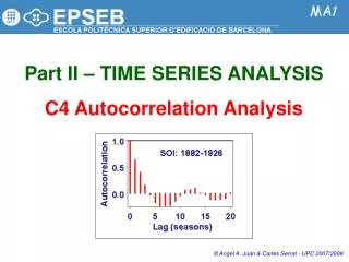
Part II – TIME SERIES ANALYSIS C4 Autocorrelation Analysis © Angel A. Juan & Carles Serrat - UPC 2007/2008
2.4.1: Lagged Values & Dependencies • Often in time series you will want to compare the value observed at one time point to a value observed one or more time points earlier. Such prior values are known as lagged values. • File: RIVERC.MTW • Stat > Time Series > Lag… You can calculate laggedvalues by letting the values in rows of the lagged column be equal to values one or more rows above in the unlagged column. In this example, it is clear that each observation is most similar (closest) to the adjacent observation (lag = 1); in addition, there is a recurring seasonal pattern, i.e., each observation is also similar to the same observation 24 hours earlier (lag = 24). It is frequent to detect a strong relationship (correlation) between the original data and some of the lagged data sets. This is specially common for the cases lag = 1 and lag = k, being k is the size of the seasonal component (k = 24 in this example).
2.4.2: Autocorrelation Function ACF (1/2) • Idea: If there is some pattern in how the values of your time series change from observations to observation, you could use it to your advantage. • The correlation between the original time series values and the corresponding k-lagged values is called autocorrelation of order k. • The Autocorrelation Function (ACF) provides the correlation between the serial correlation coefficients for consecutive lags. • Correlograms display graphically the ACF. • The ACF can be misleading for a series with unstable variance, so it might first be necessary to transform for a constant variance before using the ACF. For instance, a below-average value at time t means that it is more likely the series will be high at time t+1, or viceversa. The (1-α) confidence boundary indicates how low or high the correlation needs to be for significance at the αlevel. Autocorrelations that lie outside this range are statistically significant. For this TS, autocorrelation of order 2 (correlation between original TS data and 2-lagged data) is about 0.38.
2.4.2: Autocorrelation Function ACF (2/2) • File: RIVERC.MTW • Stat > Time Series > Autocorrelation… You can use the Ljung-Box Q (LBQ) statistic to test the null hypothesis that the autocorrelations for all lags up to lag k equal zero (the LBQ is Chi-Square distributed with df = k). Alternatively, when using α = 0.05, you can simply check whether the ACF value is beyond the significance limits. The autocorrelation plot resembles a sine pattern. This suggest that temperatures close in time are strongly and positively correlated, while temperatures about 12 hours apart are highly negatively correlated. The large positive autocorrelation at lag 24 is indicative of the 24-hour seasonal component.
2.4.3: Serial Dependency & Differencing • Note: Autocorrelations for consecutive lags are formally dependent. • Example: If the first element is closely related to the second, and the second to the third, then the first element must also be somewhat related to the third one, etc. • Implication: The pattern of serial dependencies can change considerably after removing the first order autocorrelation. • Why to remove serial dependency?: • To identify the hidden nature of seasonal dependencies in the series. • To make the series stationarywhich is necessary for ARIMA and other techniques. • How to remove it?: Serial dependency for a particular lag of k can be removed by differencing the series, that is converting each element i of the series into its difference from the element i-k. • File: RIVERC.MTW • Stat > Time Series > Differences… 2 1 3 Recall that the shape of your TS plot indicates whether the TS is stationary or nonstationary. Consider taking differences when the TS plot indicates a nonstationary time series. You can then use the resulting differenced data as your time series, plotting the differenced TS to determine if it is stationary.
2.4.4: Partial Autocorr. Function PACF (1/2) • Another useful method to examine serial dependencies is to examine the Partial Autocorrelation Function (PACF), an extension of autocorrelation where the dependence on the intermediate elements (those within the lag) is removed. • For time series data, ACF and PACF measure the degree of relationship between observations k time periods, or lags, apart. These plots provide valuable information to help you identify an appropriate ARIMA model. • In a sense, the partial autocorrelation provides a “cleaner” picture of serial dependencies for individual lags. 2 1 3 At the lag of 1 (when there are no intermediate elements within the lag), the partial autocorrelation is equivalent to autocorrelation.
2.4.4: Partial Autocorr. Function PACF (2/2) • File: RIVERC.MTW • Stat > Time Series > Partial Autocorrelation… The graph shows two large partial autocorrelations at lags 1and 2.