Download
1 / 132
1.32k likes | 1.46k Views
This lecture, led by Bhiksha Raj, delves into the process of recognizing faces in images using eigen representations. It introduces the concept of Eigenfaces, showcasing how normalized face images can be approximated using the most common features among them. The course covers techniques such as the Discrete Cosine Transform (DCT) and Singular Value Decomposition (SVD) for efficient image representation. Students will learn to compute principal components and how they can be utilized for face detection in machine learning applications.

E N D
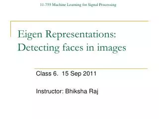
Eigen Representations:Detecting faces in images Class 6. 15 Sep 2011 Instructor: Bhiksha Raj
Administrivia • Project teams? • Project proposals? • TAs have updated timings and locations (on webpage) 11-755 MLSP: Bhiksha Raj
Last Lecture: Representing Audio • Basic DFT • Computing a Spectrogram • Computing additional features from a spectrogram 11-755 MLSP: Bhiksha Raj
What about images? Npixels / 64 columns • DCT of small segments • 8x8 • Each image becomes a matrix of DCT vectors • DCT of the image • Haar transform (checkerboard) • Or data-driven representations.. DCT 11-755 MLSP: Bhiksha Raj
Returning to Eigen Computation • A collection of faces • All normalized to 100x100 pixels • What is common among all of them? • Do we have a common descriptor? 11-755 MLSP: Bhiksha Raj
A least squares typical face The typical face • Can we do better than a blank screen to find the most common portion of faces? • The first checkerboard; the zeroth frequency component.. • Assumption: There is a “typical” face that captures most of what is common to all faces • Every face can be represented by a scaled version of a typical face • What is this face? • Approximate every face f as f = wf V • Estimate V to minimize the squared error • How? • What is V? 11-755 MLSP: Bhiksha Raj
A collection of least squares typical faces • Assumption: There are a set of K “typical” faces that captures most of all faces • Approximate every face f as f = wf,1 V1+ wf,2 V2 + wf,3 V3 +.. + wf,k Vk • V2 is used to “correct” errors resulting from using only V1 • So the total energy in wf,2 (S wf,22) must be lesser than the total energy in wf,1 (S wf,12) • V3 corrects errors remaining after correction with V2 • The total energy in wf,3 must be lesser than that even in wf,2 • And so on.. • V = [V1 V2 V3] • Estimate V to minimize the squared error • How? • What is V? 11-755 MLSP: Bhiksha Raj
A recollection M = V=PINV(W)*M ? W = U = 11-755 MLSP: Bhiksha Raj
How about the other way? M = V = ? ? W = U = • W = M * Pinv(V) 11-755 MLSP: Bhiksha Raj
How about the other way? M = ? V = ? ? W = U = • W V \approx = M 11-755 MLSP: Bhiksha Raj
Eigen Faces! M = Data Matrix • Here W, V and U are ALL unknown and must be determined • Such that the squared error between U and M is minimum • Eigen analysis allows you to find W and V such that U = WV has the least squared error with respect to the original data M • If the original data are a collection of faces, the columns of W represent the space of eigen faces. V W U = Approximation 11-755 MLSP: Bhiksha Raj
Eigen faces 300x10000 • Lay all faces side by side in vector form to form a matrix • In my example: 300 faces. So the matrix is 10000 x 300 • Multiply the matrix by its transpose • The correlation matrix is 10000x10000 M = Data Matrix 10000x10000 10000x300 Correlation = MT = TransposedData Matrix 11-755 MLSP: Bhiksha Raj
Eigen faces • Compute the eigen vectors • Only 300 of the 10000 eigen values are non-zero • Why? • Retain eigen vectors with high eigen values (>0) • Could use a higher threshold [U,S] = eig(correlation) eigenface1 eigenface2 11-755 MLSP: Bhiksha Raj
Eigen Faces eigenface1 eigenface2 • The eigen vector with the highest eigen value is the first typical face • The vector with the second highest eigen value is the second typical face. • Etc. eigenface1 eigenface2 eigenface3 11-755 MLSP: Bhiksha Raj
Representing a face • The weights with which the eigen faces must be combined to compose the face are used to represent the face! = + w2 + w3 w1 Representation = [w1w2w3 …. ]T 11-755 MLSP: Bhiksha Raj
Principal Component Analysis • Eigen analysis: Computing the “Principal” directions of a data • What do they mean • Why do we care 11-755 MLSP: Bhiksha Raj
Principal Components == Eigen Vectors • Principal Component Analysis is the same as Eigen analysis • The “Principal Components” are the Eigen Vectors 11-755 MLSP: Bhiksha Raj
Principal Component Analysis Which line through the mean leads to the smallest reconstruction error (sum of squared lengths of the blue lines) ? 11-755 MLSP: Bhiksha Raj
E2 E1 X Principal Components • The first principal component is the first Eigen (“typical”) vector • X = a1(X)E1 • The first Eigen face • For non-zero-mean data sets, the average of the data • The second principal component is the second “typical” (or correction) vector • X = a1(X)E1 + a2(X)E2 a2 a1 X = a1E1 + a2E2 11-755 MLSP: Bhiksha Raj
SVD instead of Eigen M = Data Matrix • Do we need to compute a 10000 x 10000 correlation matrix and then perform Eigen analysis? • Will take a very long time on your laptop • SVD • Only need to perform “Thin” SVD. Very fast • U = 10000 x 300 • The columns of U are the eigen faces! • The Us corresponding to the “zero” eigen values are not computed • S = 300 x 300 • V = 300 x 300 U=10000x300 S=300x300 V=300x300 10000x300 eigenface1 eigenface2 = 11-755 MLSP: Bhiksha Raj
NORMALIZING OUT VARIATIONS 11-755 MLSP: Bhiksha Raj
Images: Accounting for variations • What are the obvious differences in the above images • How can we capture these differences • Hint – image histograms.. 11-755 MLSP: Bhiksha Raj
Images -- Variations • Pixel histograms: what are the differences 11-755 MLSP: Bhiksha Raj
Normalizing Image Characteristics • Normalize the pictures • Eliminate lighting/contrast variations • All pictures must have “similar” lighting • How? • Lighting and contrast are represented in the image histograms: 11-755 MLSP: Bhiksha Raj
0 255 Histogram Equalization • Normalize histograms of images • Maximize the contrast • Contrast is defined as the “flatness” of the histogram • For maximal contrast, every greyscale must happen as frequently as every other greyscale • Maximizing the contrast: Flattening the histogram • Doing it for every image ensures that every image has the same constrast • I.e. exactly the same histogram of pixel values • Which should be flat 11-755 MLSP: Bhiksha Raj
Histogram Equalization • Modify pixel values such that histogram becomes “flat”. • For each pixel • New pixel value = f(old pixel value) • What is f()? • Easy way to compute this function: map cumulative counts 11-755 MLSP: Bhiksha Raj
Cumulative Count Function • The histogram (count) of a pixel value X is the number of pixels in the image that have value X • E.g. in the above image, the count of pixel value 180 is about 110 • The cumulative count at pixel value X is the total number of pixels that have values in the range 0 <= x <= X • CCF(X) = H(1) + H(2) + .. H(X) 11-755 MLSP: Bhiksha Raj
Cumulative Count Function • The cumulative count function of a uniform histogram is a line • We must modify the pixel values of the image so that its cumulative count is a line 11-755 MLSP: Bhiksha Raj
Mapping CCFs • CCF(f(x)) -> a*f(x) [of a*(f(x)+1) if pixels can take value 0] • x = pixel value • f() is the function that converts the old pixel value to a new (normalized) pixel value • a = (total no. of pixels in image) / (total no. of pixel levels) • The no. of pixel levels is 256 in our examples • Total no. of pixels is 10000 in a 100x100 image Move x axis levels around until the plot to the leftlooks like the plot to the right 11-755 MLSP: Bhiksha Raj
Mapping CCFs • For each pixel value x: • Find the location on the red line that has the closet Y value to the observed CCF at x 11-755 MLSP: Bhiksha Raj
Mapping CCFs • For each pixel value x: • Find the location on the red line that has the closet Y value to the observed CCF at x f(x1) = x2 f(x3) = x4 Etc. x3 x1 x4 x2 11-755 MLSP: Bhiksha Raj
Mapping CCFs • For each pixel in the image to the left • The pixel has a value x • Find the CCF at that pixel value CCF(x) • Find x’ such that CCF(x’) in the function to the right equals CCF(x) • x’ such that CCF_flat(x’) = CCF(x) • Modify the pixel value to x’ Move x axis levels around until the plot to the leftlooks like the plot to the right 11-755 MLSP: Bhiksha Raj
Doing it Formulaically • CCFmin is the smallest non-zero value of CCF(x) • The value of the CCF at the smallest observed pixel value • Npixels is the total no. of pixels in the image • 10000 for a 100x100 image • Max.pixel.value is the highest pixel value • 255 for 8-bit pixel representations 11-755 MLSP: Bhiksha Raj
Or even simpler • Matlab: • Newimage = histeq(oldimage) 11-755 MLSP: Bhiksha Raj
Histogram Equalization • Left column: Original image • Right column: Equalized image • All images now have similar contrast levels 11-755 MLSP: Bhiksha Raj
Eigenfaces after Equalization • Left panel : Without HEQ • Right panel: With HEQ • Eigen faces are more face like.. • Need not always be the case 11-755 MLSP: Bhiksha Raj
Detecting Faces in Images 11-755 MLSP: Bhiksha Raj
Detecting Faces in Images • Finding face like patterns • How do we find if a picture has faces in it • Where are the faces? • A simple solution: • Define a “typical face” • Find the “typical face” in the image 11-755 MLSP: Bhiksha Raj
Finding faces in an image • Picture is larger than the “typical face” • E.g. typical face is 100x100, picture is 600x800 • First convert to greyscale • R + G + B • Not very useful to work in color 11-755 MLSP: Bhiksha Raj
Finding faces in an image • Goal .. To find out if and where images that look like the “typical” face occur in the picture 11-755 MLSP: Bhiksha Raj
Finding faces in an image • Try to “match” the typical face to each location in the picture 11-755 MLSP: Bhiksha Raj
Finding faces in an image • Try to “match” the typical face to each location in the picture 11-755 MLSP: Bhiksha Raj
Finding faces in an image • Try to “match” the typical face to each location in the picture 11-755 MLSP: Bhiksha Raj
Finding faces in an image • Try to “match” the typical face to each location in the picture 11-755 MLSP: Bhiksha Raj
Finding faces in an image • Try to “match” the typical face to each location in the picture 11-755 MLSP: Bhiksha Raj
Finding faces in an image • Try to “match” the typical face to each location in the picture 11-755 MLSP: Bhiksha Raj
Finding faces in an image • Try to “match” the typical face to each location in the picture 11-755 MLSP: Bhiksha Raj
Finding faces in an image • Try to “match” the typical face to each location in the picture 11-755 MLSP: Bhiksha Raj
Finding faces in an image • Try to “match” the typical face to each location in the picture 11-755 MLSP: Bhiksha Raj
Finding faces in an image • Try to “match” the typical face to each location in the picture • The “typical face” will explain some spots on the image much better than others • These are the spots at which we probably have a face! 11-755 MLSP: Bhiksha Raj