Gaussian Distributions for Estimation in Robotics
350 likes | 439 Views
Understand how to combine measurements for accurate estimation, dealing with noise and uncertainties using Gaussian distributions. Learn about the Kalman filter for optimal recursive data processing in robot state estimation.

Gaussian Distributions for Estimation in Robotics
E N D
Presentation Transcript
Probability, Gaussians andEstimation David Johnson
Basic Problem • Approaches so far • Robot state is a point in state space • q = ( x, y, vx, vy, heading ) • This state based on measurements • External (GPS, beacons, vision) • Internal (odometry, gyros) • Measurements not exact • Errors can accumulate • How to “clean” measurements • filtering • How to combine measurements? • estimation
Problems to solve • Localization • Given a map where am I? • Mapping • Given my position, build a map • SLAM – Simultaneous Localization and Mapping • Drop down a robot, build a map and location within in at the same time
Approach • Treat state variables as probabilities • Combine measurements weighted by reliability • Use filtering to improve estimate of state
Example - Triangulation • Time of flight from beacons gives distance • Constrains to a circle • 2 beacons to point solutions
Noise in Measurements • Uncertainty in measurement • Can be reported as plus/minus some value • Creates solution regions • Even this is a simplification • Measurements follow a distribution
Coin Flip • F=(head, tails) • Discrete distribution • Probability of a coin flip being head or tails is 0.5 + 0.5 = 1 • But what about continuous distributions? • Probability someone in the room is exactly 2 meters tall is infinitesimal • Talk about probability of intervals instead
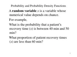
f(x) x Continuous distributions • Probability density function f(x) • Find probability of a measurement being within an interval • What is f(x) for a uniform distribution over range [u,v]?
Gaussian distributions • Bell-shaped f(x) • Can assume most measurements with noise follow a Gaussian distribution • Why • Central Limit Theorem • Applet
p ( x ) ~ Ν ( μ , Σ ) : 1 1 - t 1 - - - x μ Σ x μ ( ) ( ) = p ( x ) e 2 1 / 2 p d / 2 ( 2 ) Σ Gaussian Definition m s 2 p ( x ) ~ N ( , ) : 2 - m 1 ( ) x 1 m - = 2 s 2 p ( x ) e p s 2 Univariate -s s m Multivariate
Discrete Variance vs Continuous • Discrete • Continuous
Gaussians • Gaussians completely described by mean and variance • Non-zero mean implies a bias in measurement • Zero mean can be removed by filtering
Filtering • Gaussian noise = N(0, ) • Make repeated measurements • Histogram the samples • Find the peak – that is the mean • Easy! • What is the size of the whiteboard in meters (1 decimal place precision)? s 2
Non-static situation • What happens when state evolves? • Can’t repeat measurements • Moving average filter • Introduces lag into system!
Use a state model • Estimate position from measurements • Measure velocity as well • Evolve position from velocity • Incorporate evolved state into position measurements • Need to combine multiple, uncertain measurements
Back to the non-evolving case • Two different processes measure the same thing • Want to combine into one better measurement • Estimation
Estimator Data + noise Data + noise Data + noise Estimation Estimation What is meant by estimation? z estimate H ŷ Stochastic process
A Least-Squares Approach • We want to fuse these measurements to obtain a new estimate for the range • Using a weighted least-squares approach, the resulting sum of squares error will be • Minimizing this error with respect to yields
A Least-Squares Approach • Rearranging we have • If we choose the weight to be • we obtain
A Least-Squares Approach • For merging Gaussian distributions, the update rule is Show for N(0,a) N(0,b)
Kalman Gain A Least-Squares Approach • This can be rewritten as • or if we think of this as adding a new measurement to our current estimate of the state we would get • For merging Gaussian distributions, the update rule is • which if we write in our measurement update equation form we get show
What happens when you move? derive
Moving • As you move • Uncertainty grows • Need to make new measurements • Combine measurements using Kalman gain
OPTIMAL: • Linear dynamics • Measurements linear w/r to state • Errors in sensors and dynamics must be zero-mean (un-bias) white Gaussian • RECURSIVE: • Does not require all previous data • Incoming measurements ‘modify’ current estimate The Kalman Filter DATA PROCESSING ALGORITHM: The Kalman filter is essentially a technique of estimation given a system model and concurrent measurements (not a function of frequency) “an optimal recursive data processing algorithm”
Estimate the state of a discrete-time controlled process that is governed by the linear stochastic difference equation: with a measurement: The random variables wk and vk represent the process and measurement noise (respectively). They are assumed to be independent (of each other), white, and with normal probability distributions In practice, the process noise covariance and measurement noise covariance matrices might change with each time step or measurement. The Discrete Kalman Filter (PDFs)
State transition Control signal The Discrete Kalman Filter State prediction “prior” estimate Process noise covariance First part – model forecast: prediction Error covariance prediction Prediction is based only the model of the system dynamics.
actual measurement “prior” state prediction The Discrete Kalman Filter state correction Kalman gain predicted measurement “posterior” estimate update error covariance matrix (posterior) Second part – measurement update: correction
variance of the predicted states = ------------------------------------------------------------ variance of the predicted + measured states The Discrete Kalman Filter measurement sensitivity matrix measurement noise covariance The Kalman gain, K:“Do I trust my model or measurements?”
Estimate a constant voltage • Measurements have noise • Update step is • Measurement step is