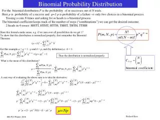
Binomial probability estimation
Binomial probability estimation. Playing chess against a friend you won 3 out of 5 matches and lost 2. Assuming that wins and losses follow the binomial distribution: What is the probability that you will win the next match? What is the probability distribution of the results of the next match?

Binomial probability estimation
E N D
Presentation Transcript
Binomial probability estimation • Playing chess against a friend you won 3 out of 5 matches and lost 2. Assuming that wins and losses follow the binomial distribution: • What is the probability that you will win the next match? • What is the probability distribution of the results of the next match? • Assuming that you will be playing many games with your friend, and that your probability of winning will not change, what is the median of your expected probability of winning and what are the 95% confidence limits of that figure?
Solution • Probability of winning the next match • Probability distribution for next match • P(y=1)=0.571, P(y=0)=0.429. • Median • mybeta=@(x) betacdf(x,4,3)-0.5 • medi=fzero(@(x) mybeta(x), 0.5)=0.5786 • medicheck=betainv(0.5,4,3)=0.5786 • Confidence bounds • low=betainv(0.025,4,3)=0.2228 • high=betainv(0.975,4,3)=0.8819
Known variance with one sample • For standard normal, get one sample and plot true, posterior and predictive. • Repeat with 10 samples
One sample x=linspace(-5,5,501); true=normpdf(x,0,1); samp=randn(1,1)=-1.3077 poster=normpdf(x,samp,1); predict=normpdf(x,sampe,sqrt(2)); plot(x,true,x,poster,'r',x,predict,'g') legend('true','posterior','predictive','Location','NorthEast') xlabel('x'); ylabel('pdf') What is different about the red curve as compared to the other two?
10 samples y=randn(1,10); mu=mean(y)=-0.5038 poster=normpdf(x,mu,sqrt(0.1)); sig=sqrt(1.1); predict=normpdf(x,mu,sig); .
Known mean • Use the same 10 samples to plot the true, posterior, and predictive distributions when the mean is known to be zero, but we need to estimate the distribution of the variance. • Because we do not have a formula for the predictive distribution do it by simulation.
Variance with known mean • With the known mean we use for the variance • Matlab divides by n-1, which corresponds to estimated mean std2=std(y)^2=0.7636 var=sum((y-mu).^2)/10 var=0.6873 varcheck=std2*(9/10) varcheck=0.6873
Posterior pdf and cdf sig2x=linspace(0.01,5,500); z=10*var./sig2x; poster=(z./sig2x).*chi2pdf(z,10); plot(sig2x, poster) area=mean(poster)*5=0.9993 postcdf=1.-chi2cdf(z,10); hold on plot(sig2x,postcdf,'r') xlabel('\sigma2') legend('pdf','cdf') .
Sampling from the sig2 distribution • Increment makes the cdf monotonic and corrects the final value from 0.9993 to 1. • When the CDF is known, we sample uniformly in [0,1] and take the x corresponding to that CDF value. • We now sample from normal distribution with a mean of zero and a standard deviation that corresponds to the sig2 sample. • We check the mean and standard deviation increment=linspace(0,0.0007,500); postcdf=postcdf+increment; p=rand(1,10000); sig2p=interp1(postcdf,sig2x,p); sample=randn(1,10000).*sqrt(sig2p); mean(sample)=8.8362e-04 std(sample)=0.9114