Download
1 / 15
150 likes | 247 Views
Comparison of data from Wind and SSX experiments using various analysis techniques to study helicity, delays, embedding, and permutation metrics.

E N D
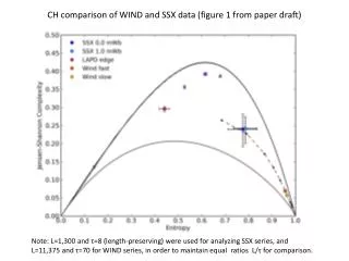
CH comparison of WIND and SSX data (figure 1 from paper draft) Note: L=1,300 and τ=8 (length-preserving) were used for analyzing SSX series, and L=11,375 and τ=70 for WIND series, in order to maintain equal ratios L/τ for comparison.
Helicity Scan for length-preserving delay 8, channel 1 Bdotdata (figure 2 from draft)
Delay scan 1 to 150 for B and B-dot data, first 4 channels (figure 3 from draft)
Embedding delay scan 9 to 875 for WIND fast stream B_x series, averaged over 20 sections of 11375 values (i.e. normalized to same L/τ range as SSX data in prior plot)
Embedding delay scan 9 to 438 for WIND fast stream B_x series, averaged over 20 sections of 11375 values (i.e. normalized to same L/τ range as SSX data up to τ= 50)
Differences between permutation metrics averaged over 1,000 value sections of slow & fast WIND B_x series as functions of delay τ (thought to be artificial effects)
CH planes for WIND ensemble averages over 1,000 value sections τ = 10 τ = 20 τ = 50 τ = 100
CH planes for ensemble averages over sections with L/τ equal to ratio for SSX (162.5) τ = 10 τ = 20 τ = 50 τ = 100
Delay dependence of PE_fastx, C_fastx, and C_slowx- C_fastx averaged over sections of lengths L such that L / τ = 162.5 (as for SSX)
CH comparison of SSX, WIND, and LAPD data (p0 and p30 unbiased) Note: L=1,300 and τ=8 were used for analyzing SSX series, and L=11,375 and τ=70 for WIND series, in order to maintain equal ratios L/τ for comparison.
CH comparison of SSX, WIND, and LAPD data, using τ = 10 for LAPD data
Embedding delay scan 1 to 100 for LAPD core data (blue) and edge (Red) Each point represents an average over 25 shots.
Embedding delay scan 1 to 100 for reduced LAPD core data (blue) and edge (Red) Reduced series consist of first half (2500 values) of original
Comparison of SSX B from integration, from fft method, and Bdot for 0.75 mWb Note: τ=8 were used for all SSX series. Analysis was run on 40-60 microsecond window, only for first four channels. Scatter is over 3 directions, 40 shots, 4 channels.