Maximum Covariance Analysis
Maximum Covariance Analysis. Canonical Correlation Analysis. FIG. 6. The CCA mode 1 for (a) SLP and (b) SST . The pattern in (a) is scaled by [max(u )-min (u)]/2, and (b) by [max ( v )-min( v ) ]/2 . Contour interval is 0.5 mb in (a) and 0.5C in (b).


Maximum Covariance Analysis
E N D
Presentation Transcript
Maximum Covariance Analysis Canonical Correlation Analysis
FIG. 6. The CCA mode 1 for (a) SLP and (b) SST. The pattern in (a) is scaled by [max(u)-min(u)]/2, and (b) by [max(v)-min(v)]/2. Contour interval is 0.5 mb in (a) and 0.5C in (b). Hsieh, W. (2001) Nonlinear Canonical Correlation Analysis of the Tropical Pacific Climate Variability Using a Neural Network Approach, J. Climate, 14, 2528-2539
FIG. 12. The CCA mode 2 for (a) SLP and (b) SST. Contour interval is 0.2 mb in (a) and 0.2C in (b). Hsieh, W. (2001) Nonlinear Canonical Correlation Analysis of the Tropical Pacific Climate Variability Using a Neural Network Approach, J. Climate, 14, 2528-2539
Statistical downscaling 14.3.3 North Atlantic SLP and Iberian Rainfall: Analysis and Historic Reconstruction In this example, winter (DJF) mean precipitation from a number of rain gauges on the Iberian Peninsula is related to the air-pressure field over the North Atlantic. CCA was used to obtain a pair of canonical correlation pattern estimates (Figure 14.4), and corresponding time series of canonical variate estimates. These strongly correlated modes of variation (the estimated canonical correlation is 0.75) represent about 65% and 40% of the total variability of seasonal mean SLP and Iberian Peninsula precipitation respectively. The two patterns represent a simple physical mechanism: when SLP mode 1 has a strong positive coefficient, enhanced cyclonic circulation advects more maritime air onto the Iberian Peninsula so that precipitation in the mountainous northwest region (precip mode 1) is increased. Since the canonical correlation is large, the results of the CCA can be used to forecast or specify winter mean precipitation on the Iberian peninsula from North Atlantic SLP. Von Storch, H., and F. W. Zwiers(2002) Statistical analysis in climate research, Cambridge University Press.
14.3.3 North Atlantic SLP and Iberian Rainfall: Analysis and Historic Reconstruction The analysis described above was performed with the 1950-80 segment of a data set that extends back to 1901. Since the 1901-49 segment is independent of that used to 'train' the model, it can be used to validate the model Figure 14.5 shows both the specified and observed winter mean rainfall averaged over all Iberian stations for this period. The overall upward trend and the low-frequency variations in observed precipitation are well reproduced by the indirect method indicating the usefulness of the technique as well as the reality of both the trend and the variations in the Iberian winter precipitation.
14.3.4 North Atlantic SLP and Iberian Rainfall: Downscaling of GCM output This regression approach has an interesting application in climate change studies. GCMs are widely used to assess the impact that increasing concentrations of greenhouse gases might have on the climate system. But, because of their resolution, GCMs do not represent the details of regional climate change well. The minimum scale that a GCM is able to resolve is the distance between two neighboring grid points whereas the skillful scale is generally accepted to be four or more grid lengths. The minimum scale in most climate models in the mid 1990s is of the order of 250-500 km so that the skillful scale is at least 1000-2000 km. Thus the scales at which GCMs produce useful information does not match the scale at which many users, such as hydrologists, require information. Statistical downscaling is a possible solution to this dilemma. The idea is to build a statistical model from historical observations that relates large-scale information that can be well simulated by GCMs to the desired regional scale information that can not be simulated. These models are then applied to the large-scale model output. • The following steps must be taken. • 1. Identify a regional climate variable R of • Interest • 2. Find a climate variable L that: • controls R in the sense that there is a statistical relationship between Rand Lof the form R = G(L,a) + e in which G(L,a)represents a substantial fraction of the total variance of R. Vector a contains parameters that can be used to adjust the fit • is reliably simulated in a climate model. • 3. Use historical realizations of (R, L) to estimate a. • 4. Validate the fitted model on independent historical data • 5. Apply the validated model to GCM simulated realizations of L.
This are exactly the steps taken in the Atlantic SLP and Iberian precipitation analysis. A statistical model was constructed that related Iberian rainfall Rto North Atlantic SLP L through a simple linear functional. The adjustable parameters a consisted of the canonical correlation patterns. These parameters were estimated from 1950 to 1980 data. Observations before 1950 were used to validate the model. The downscaling model was applied to the output of a 2xC02experiment performed with a GCM. Figure 14.6 compares the 'downscaled’ response to doubled C02 with the model's grid point response. The latter suggests that there will be a marked decrease in precipitation over most of the Peninsula whereas the downscaled response is weakly positive. The downscaled response is physically more reasonable than the direct response of the model.
In relatively high-dimensional x and y spaces, among the many dimensions and using correlations calculated with relatively small samples, CCA can often find directions of high correlation but with little variance, thereby extracting a spurious leading CCA mode, as illustrated. Figure: With the ellipses denoting the data clouds in the two input spaces, the dotted lines illustrate directions with little variance but by chance with high correlation (as illustrated by the perfect order in which the data points 1, 2, 3 and 4 are arranged in the x and y spaces). Since CCA finds the correlation of the data points along the dotted lines to be higher than that along the dashed lines (where the data points a, b, c and d in the x-space are ordered as b, a, d and c in the y-space), the dotted lines are chosen as the first CCA mode. Maximum covariance analysis (MCA), looks for modes of maximum covariance instead of maximum correlation, and would select the dashed lines over the dotted lines since the length of the lines do count in the covariance but not in the correlation. It can be shown that the MCA problem can be derived from CCA by pre-filtering the data using Principal Components (EOFs) of the data. But a more straightforward derivation is obtained using a different normalization before using the method of Lagrange multipliers.