Download
1 / 36
380 likes | 788 Views
Slides 13b: Time-Series Models; Measuring Forecast Error. MGS3100 Chapter 13. Forecasting. Forecasting Models. Time Series Models . General Form: Y = T * C * S ± ε, where T = Trend - long term movement of mean

E N D
Slides 13b: Time-Series Models;Measuring Forecast Error MGS3100 Chapter 13 Forecasting
Time Series Models • General Form: Y = T * C * S ± ε, where • T = Trend - long term movement of mean • C = (Business) Cycle - an upturn or downturn not caused by seasonal variation; effect of the economy • S = Seasonal Variation - repetitive pattern observed over a specific time period • ε = Error (random variation) • Practical Forecast Form: Ŷ = T * S • C is important, but difficult to forecast • Don’t forecast an error!
Components of a Time Series Time series value Linear trend and seasonality time series Future Linear trend time series A stationary time series Time
Time Series: Stationary Models • Stationary Model Assumptions • Assumes item forecasted will stay steady over time (constant mean; random variation only) • Techniques will smooth out short-term irregularities • Forecast for period t+1 is equal to forecast for period t+k; the forecast is revised only when new data becomes available. • Stationary Model Types • Naïve Forecast • Moving Average • Weighted Moving Average • Exponential Smoothing
Stationary Time Series Models:The Naïve Model • Whatever happened last period will happen again this time • The model is simple and flexible • Provides a baseline to measure other models • Attempts to capture seasonal factors at the expense of ignoring trend or
Measures of Forecast Error • Bias - The arithmetic sum of the errors • MAD - Mean Absolute Deviation • MAPE – Mean Absolute Percentage Error • Mean Square Error (MSE) - Similar to simple sample variance • Standard Error - Standard deviation of the sampling distribution (the square root of the MSE) • Bias, MAD, and MAPE - typically used for time series
Stationary Time Series Models:Moving Averages • The Moving Average Method • The forecast is the average of the last n observations of the time series.
Stability vs. Responsiveness • Should I use a 2-period moving average or a 3-period moving average? • The larger the “n” the more stable the forecast. • A 2-period model will be more responsive to change. • We don’t want to chase outliers. • But we don’t want to take forever to correct for a real change. • We must balance stability with responsiveness.
Stationary Time Series Models:Weighted Moving Averages • The Weighted Moving Average Method • Historical values of the time series are assigned different weights when performing the forecast = w1Yt + w2Yt-1 +w3Yt-2 + …+ wnYt-n+1 Swi = 1
Stationary Time Series Models:Exponential Smoothing • Exponential Smoothing • Moving average technique that requires a minimum amount of past data • Uses a smoothing constant α with a value between 0 and 1 (Usual range 0.1 to 0.3) • Forecast for period t = Forecast for period t-1 plus α times the difference between the actual value and forecast in period t-1: Ŷt = Ŷt-1 + α(Yt-1 - Ŷt-1), or • Can also be expressed as: Ŷt = α(Yt-1) + (1- α)(Ŷt-1) = α(Actual value in period t-1) + (1- α)(Forecast in period t-1)
Exponential Smoothing Data Class Exercise: What is the forecast for January of the following year? How about March? Find the Bias, Mad & MAPE. (Note: α equals 0.1.)
Evaluating the Performance of Forecasting Techniques • Several forecasting methods have been presented. • Which one of these forecasting methods gives the “best” forecast?
Performance Measures – Sample Example Time 1 2 3 4 5 6 Time series: 100 110 90 80 105 115 3-Period Moving average: 100 93.33 91.6 Error for the 3-Period MA: - 20 11.67 23.4 3-Period Weighted MA(.5, .3, .2) 98 89 85.5 Error for the 3-Period WMA - 18 16 29.5 • Find the forecasts and the errors for each forecasting technique applied to the following stationary time series.
MAD for the moving average technique: |-20| + |11.67| + |23.4| 3 |D t| n |D t| n S S MAD = = MAD = = MAD for the weighted moving average technique: |-18| + |116| + |29.5| 3 Performance Measures –MAD for the Sample Example = 18.35 = 21.17
MAPE for the moving average technique: |-20|/80 + |11.67|/105+ |23.4|/115 3 |D t| n |D t| n S S MAPE= = MAPE= = MAPE for the weighted moving average technique: |-18|/80 + |16|/105 + |29.5|/115 3 Performance Measures – MAPE for the Sample Example = .188 = .211
Performance Measures –Selecting Model Parameters • Use the performance measures to select a good set of values for each model parameter. • For the moving average: • the number of periods (n). • For the weighted moving average: • The number of periods (n), • The weights (wi). • For the exponential smoothing: • The exponential smoothing factor (a). • Excel Solver can be used to determine the values of the model parameters.
Trend & Seasonality • Trend analysis • Technique that fits a trend equation (or curve) to a series of historical data points • Projects the equation into the future for medium and long term forecasts. Typically do not want to forecast into the future more than half the number of time periods used to generate the forecast • Seasonality analysis • Adjustment to time series data due to variations at certain periods. • Adjust with seasonal index - ratio of average value of the item in a season to the overall annual average value. • Examples: demand for coal in winter months; demand for soft drinks in the summer and over major holidays
Least Squares for Linear RegressionMidwestern Manufacturing Objective: Minimize the squared deviations!
Least Squares Method Where = predicted value of the dependent variable (demand) X = value of the independent variable (time) a = Y-axis intercept = - b* b = Slope of the regression line =
Another way to Determine Trend:Use the Excel Regression Function • Run linear regression to test b1 in the model Yt=b0+b1t+et • Excel results: 0.71601 This large P-value indicates that there is little evidence that trend exists • Conclusion: A stationary model is appropriate.
Forecasting Seasonal Data: Quick Method Ratio = Demand / Average Demand Seasonal Index – ratio of the average value of the item in a season to the overall average annual value. Example: average of year 1 January ratio to year 2 January ratio. (0.851 + 1.064)/2 = 0.957 If Year 3 average monthly demand is expected to be 100 units. Forecast demand Year 3 January: 100 X 0.957 = 96 units Forecast demand Year 3 May: 100 X 1.309 = 131 units
Forecasting Seasonal Data With Trend • Calculate the seasonal indices (as shown on the previous slide) • Calculate “deseasonalized” treand by dividing the actual value (Y) by the seasonal index for that period: Deseasonalized Trend = Y / Seasonal index(e.g., 80 units/ 0.957 = 83.595) • Find the trend line, and extend the trend line into the desired forecast period.
Forecasting Seasonal Data With Trend: Calculating the Seasonal Forecast 4.Now that we have the Seasonal Indices and Trend line, we can reseasonalize the data and generate the “seasonalized” forecast by multiplying the trend line values in the forecast period by the appropriate seasonal indices for each time period as follows: Ŷ = Trend x Seasonal Index