Abbreviated Interrupted Time-Series
1.08k likes | 1.32k Views
Abbreviated Interrupted Time-Series. What is Interrupted Time Series (ITS)? Rationales Designs Analysis. What is ITS?. A series of observations on the same dependent variable over time

Abbreviated Interrupted Time-Series
E N D
Presentation Transcript
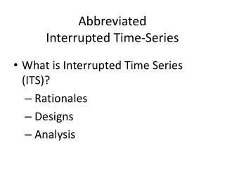
Abbreviated Interrupted Time-Series • What is Interrupted Time Series (ITS)? • Rationales • Designs • Analysis
What is ITS? • A series of observations on the same dependent variable over time • Interrupted time series is a special type of time series where treatment/intervention occurred at a specific point and the series is broken up by the introduction of the intervention. • If the treatment has a causal impact, the post-intervention series will have a different level or slope than the pre-intervention series
The effects of charging for directory assistance in Cincinnati Intervention
The effects of an alcohol warning label on prenatal drinking Label Law Date Impact Begins
Interrupted Time Series Can Provide Strong Evidence for Causal Effects • Clear Intervention Time Point • Huge and Immediate Effect • Clear Pretest Functional Form + many Observations • No alternative Can Explain the Change
How well are these Conditions met in Most Ed Research? • The Box & Jenkins tradition require roughly 100 observations to estimate cyclical patterns and error structure, but • This many data points is rare in education, and so we will have to deviate (but borrow from) the classical tradition. • Moreover,…
Meeting ITS Conditions in Educational Research • Long span of data not available and so the pretest functional form is often unclear • Implementing the intervention can span several years • Instantaneous effects are rare • Effect sizes are usually small • And so the need arises to develop methods for abbreviated time series and to supplement them with additional design features such as a control series to help bolster the weak counterfactual associated with a short pretest time series
Abbreviated Interrupted Time Series • We use abbreviated ITS loosely • series with only 6 to 50 time points • Pretest time points are important • valuable for estimating pre-intervention growth (maturation) • control for selection differences if there is a comparison time series • Posttest for identifying nature of the response, especially its temporal persistence
Theoretical Rationales for more Pretest Data Points in SITS • O X O • Describes starting level/value - yet fallibly so because of unreliability • But pre-intervention individual growth is not assessed, and this is important in education
O O X O • Describes initial standing more reliably by averaging the two pretest values • Describes pre-intervention growth better, but even so it is still only linear growth • Cannot describe stability of this individual linear growth estimate
O O O X O • Initial standing assessed even more reliably • Individual growth model can be better assessed—allow functional form to be more complex, linear and quadratic • Can assessed stability of this individual growth model (i.e., variation around linear slope)
Generalizing to 00000000X0 • Stable assessment of initial mean and slope and cyclical patterns • Estimation of reliability of mean and slope • Help determine a within-person counterfactual • Check whether anything unusual is happening before intervention
Threats to Validity: History • With most simple ITS, the major threat to internal validity is history—that some other event occurred around the same time as the intervention and could have produced the same effect. • Possible solutions: • Add a control group time series • Add a nonequivalent dependent variable • The narrower the intervals measured (e.g., monthly rather than yearly), the fewer the historical events that can explain the findings within that interval.
Threats to Validity: Instrumentation • Instrumentation: the way the outcome was measured changed at the same time that the intervention was introduced. • In Chicago, when Orlando Wilson took over the Chicago Policy Department, he changed the reporting requirements, making reporting more accurate. The result appeared to be an increase in crime when he took office. • It is important to explore the quality of the outcome measure over time, to ask about any changes that have been made to how measurement is operationalized.
Threat to SCV • When a treatment is implemented slowly and diffusely, as in the alcohol warning label study, the researcher has to specify a time point at which the intervention “took effect” • Is it the date the law took effect? • Is it a later date (and if so, did the researcher capitalize on chance in selecting that date)? • Is it possible to create a “diffusion model” instead of a single date of implementation?
Construct Validity • Reactivity threats (due to knowledge of being studied) are often less relevant if archival data are being used. • However, the limited availability of a variety of archival outcome measures means the researcher is often limited to studying just one or two outcomes that may not capture the real outcomes of interest very well
External Validity • The essence of external validity is exploring whether the effect holds over different units, settings, outcome measures, etc. • In ITS, this is only possible if the time series can be disaggregated by such moderators, which is often not the case.
O X OO O • Now we add a comparison group that did not receive treatment and we can • Assess how the two groups differ at one pretest • But only within limits of reliability of test • Have no idea how groups are changing over time
O O X O O O O • Now can test mean difference more stably • Now can test differences in linear growth/change • But do not know reliability of each unit’s change • Or of differences in growth patterns more complex than linear
O O O X O O O O O • Now mean differences more stable • Now can examine more than differences in linear growth • Now can assess variation in linear change for each unit and for group • Now can see if final pre-intervention point is an anomaly relative to earlier two
Example from Education: Project Hope • A merit-based financial aid program in Georgia • Implemented in 1993 • Cutoff of a 3.0 GPA in high school (RDD?) • Aimed to improve • Access to higher education • Educational outcomes • Control Groups • US data • Southeast data
Results: Percent of Students Obtaining High School GPA 3.00 Percent of Students Reporting B or Better 90.00% 88.00% 86.00% Southeast 84.00% 82.00% US Percent 80.00% GA 78.00% 76.00% 74.00% 90 92 94 96 98 2000 Year
Results: Average SAT scores for students reporting high school GPA 3.00
Adding a nonequivalent dependent variable to the time series NEDV: A dependent variable that is predicted not to change because of treatment, but is expected to respond to some or all of the contextually important internal validity threats in the same way as the target outcome
Example: British Breathalyzer Experiment • Intervention: A crackdown on drunk driving using a breathalyzer. • Presumed that much drunk driving occurred after drinking at pubs during the hours pubs were open. • Dependent Variable: Traffic casualties during the hours pubs were open. • Nonequivalent Dependent Variable: Traffic casualties during the hours pubs were closed. • Helps to reduce the plausibility of history threats that the decrease was due to such things as: • Weather changes • Safer cars • Police crackdown on speeding
Note that the outcome variable (open hours on weekend) did show an effect, but the nonequivalent dependent variable (hours when clubs were closed) did not show an effect.
Example: Media Campaign to Reduce Alcohol Use During a Student Festival at a University (McKillip) • Dependent Variable: Awareness of alcohol abuse. • Nonequivalent Dependent Variables (McKillip calls them “control constructs”): • Awareness of good nutrition • Awareness of stress reduction • If the effect were due to secular trends (maturation) toward better health attitudes in general, then the NEDVs would also show the effect.
Only the targeted dependent variable, awareness of responsible alcohol use, responded to the treatment, suggesting the effect is unlikely to be due to secular trends in improved health awareness in general Campaign
Adding more than one nonequivalent dependent variable to the design of SITS to increase internal validity
NCLB • National program that applies to all public school students and so no equivalent group for comparison • We can use SITS to examine change in student test score before and after NCLB • Increase internal validity of causal effect by using 3 possible types of non-equivalent groups or 3 types of contrasts for comparison
Contrast Type 1 & 2 • Contrast 1: Test for NCLB effect nationally • Compare student achievement in public schools with private schools (both Catholic and non-Catholic) • Contrast 2: Test for NCLB effects at the state level • Compare states varying in proficiency standards. • States with higher proficiency standards are likely to have more schools fail to make AYP and so more schools will need to “reform” to boost student achievement
Contrast 1: Public vs Private Schools • Public schools got NCLB but private ones essentially did not • If NCLB is raising achievement in general, then public schools should do better than private ones after 2002 • Hypothesis is that changes in mean, slope or both after 2002 will favor public schools
Hypothetical NCLB effects on public (red) versus private schools (blue) NAEP Test Score 208 200 NCLB Time
Contrast 1: Public vs Private Schools • Two independent datasets: Main and Trend NAEP data can be used to test this • Main NAEP four posttest points. Data available for both Catholic and other private schools • Trend NAEP only one usable post-2002 point and then only for Catholic schools
Analytic Model • NCLB Public vs. Catholic school contrast • Model • Low Power • Only 3 groups (public, Catholic, non-Catholic private) with 8 time points. So only 24 degrees of freedom • Autocorrelation • Few solutions • Cannot use clustering algorithm because there are not enough groups • Robust s.e. used but results less conservative
Main NAEP Time Series Graphs Public vs. Catholic Public vs. Other Private
Main NAEP 4th grade math scores by year: Public and Catholic schools
Main NAEP 4th grade math scores by year: Public and Other Private schools
Difference in differences in Total change for 4th Grade Math Analyses based on Main NAEP data
Main NAEP 8th grade math scores by year: Public and Catholic schools
Main NAEP 8th grade math scores by year: Public and Other Private schools
Difference in differences in Total change for 8th Grade Math Analyses based on Main NAEP data
Trend NAEP Time Series Graphs Public vs. Catholic School Contrast (Other private school data unavailable and only 1 post-intervention time point)
Trend NAEP 4th grade math scores by year: Public and Catholic schools