Download
1 / 43
780 likes | 1.34k Views
Geophysical Inverse Problems with a focus on seismic tomography. CIDER2012- KITP- Santa Barbara. Seismic travel time tomography. Principles of travel time tomography. 1) In the background, “reference” model: Travel time T along a ray g:. v 0 (s) velocity at point s on the ray

E N D
Geophysical Inverse Problemswith a focus on seismic tomography CIDER2012- KITP- Santa Barbara
Principles of travel time tomography 1) In the background, “reference” model: Travel time T along a ray g: v0(s) velocity at point s on the ray u= 1/v is the “slowness” The ray path g is determined by the velocity structure using Snell’s law. Ray theory. 2) Suppose the slowness u is perturbed by an amount du small enough that the ray path g is not changed. The travel time is changed by:
lij is the distance travelled by ray i in block j v0j is the reference velocity (“starting model”) in block j Solving the problem: “Given a set of travel time perturbations dTi on an ensemble of rays {i=1…N}, determine the perturbations (dv/v0)j in a 3D model parametrized in blocks (j=1…M}” is solving an inverse problem of the form: d= data vector= travel time pertubations dT m= model vector = perturbations in velocity
G has dimensions M x N Usually N (number of rays) > M (number of blocks): “over determined system” We write: GTG is a square matrix of dimensions MxM If it is invertible, we can write the solution as: where (GTG)-1 is the inverse of GTG In the sense that (GTG)-1(GTG) = I, I= identity matrix “least squares solution” – equivalent to minimizing ||d-Gm||2
“””least squares solution” Minimizes ||d-Gm||2 • G contains assumptions/choices: • Theory of wave propagation (ray theory) • Parametrization (i.e. blocks of some size) In practice, things are more complicated because GTG, in general, is singular: Some Gij are null ( lij=0)-> infinite elements in the inverse matrix
How to choose a solution? • Special solution that maximizes or minimizes some desireable property through a norm • For example: • Model with the smallest size (norm): mTm=||m||2=(m12+m22+m32+…mM2)1/2 • Closest possible solution to a preconceived model <m>: minimize ||m-<m>||2 regularization
Minimize some combination of the misfit and the solution size: • Then the solution is the “damped least squares solution”: e=d-Gm Tikhonov regularization
We can choose to minimize the model size, • eg ||m||2 =[m]T[m] - “norm damping” • Generalize to other norms. • Example: minimize roughness, i.e. difference between adjacent model parameters. • Consider ||Dm||2instead of ||m||2and minimize: • More generally, minimize: <m> reference model
Weighted damped least squares • More generally, the solution has the form: For more rigorous and complete treatment (incl. non-linear): See Tarantola (1985) Inverse problem theory Tarantola and Valette (1982)
Concept of ‘Generalized Inverse’ • Generalized inverse (G-g) is the matrix in the linear inverse problem that multiplies the data to provide an estimate of the model parameters; • For Least Squares • For Damped Least Squares • Note : Generally G-g≠G-1
As you increase the damping parameter e, more priority is given to model-norm part of functional. • Increases Prediction Error • Decreases model structure • Model will be biased toward smooth solution • How to choose e so that model is not overly biased? • Leads to idea of trade-off analysis. “L curve” η
Model Resolution Matrix • How accurately is the value of an inversion parameter recovered? • How small of an object can be imaged ? • Model resolution matrix R: • R can be thought of as a spatial filter that is applied to the true model to produce the estimated values. • Often just main diagonal analyzed to determine how spatial resolution changes with position in the image. • Off-diagonal elements provide the ‘filter functions’ for every parameter.
Checkerboard test 80% R contains theoretical assumptions on wave propagation, parametrization And assumes the problem is linear After Masters, CIDER 2010
Ingredients of an inversion • Importance of sampling/coverage • mixture of data types • Parametrization • Physical (Vs, Vp, ρ, anisotropy, attenuation) • Geometry (local versus global functions, size of blocks) • Theory of wave propagation • e.g. for travel times: banana-donut kernels/ray theory
P, PP • S, SS • Arrivals well separated on the • seismogram, suitable for travel • time measurements • Generally: • Ray theory • Iterative back projection • techniques • - Parametrization in blocks Surface waves SS S P 50 mn
P velocity tomography ...and plumes Slabs…… Van der Hilst et al., 1998 Montelli et al., 2004
P Travel Time Tomography: Ray Density maps Vasco and Johnson,1998
Checkerboard tests Karason and van der Hilst, 2000
05 11 Honshu 06 12 Fukao and Obayashi 2011 410 410 660 660 ±1.5 % 1000 07 ±1.5 % 13 13 northern Bonin 08 14 09 15 15
06 11 07 12 Tonga 410 660 ±1.5% 1000 13 08 ±1.5% Kermadec 09 14 15 10 Fukao and Obayashi 2011
Fukao and Obayashi, 2011 400 660 1000 South Pacific superswell Tonga EPR S40RTS Ritsema et al., 2011 PRI-S05 Montelli et al., 2005
Rayleigh waveovertones By including overtones, we can see into the transition zone and the top of the lower mantle. after Ritsema et al, 2004
Models from different data subsets 120 km 600 km 1600 km 2800 km After Ritsema et al., 2004
The travel time dataset in this model includes: Sdiff ScS2 Multiple ScS: ScSn
Coverage of S and P After Masters, CIDER 2010
SS Surface waves S P
Full Waveform Tomography • Long period (30s-400s) 3- component seismic waveforms • Subdivided into wavepackets and compared in time domain to synthetics. • u(x,t) = G(m) du = A dm • A= ∂u/∂m contains Fréchet derivatives of G UC B e r k e l e y
SS Sdiff PAVA NACT Li and Romanowicz , 1995
PAVA NACT
2800 km depth from Kustowski, 2006 Waveforms only, T>32 s! 20,000 wavepackets NACT
Indian Ocean Paths - Sdiffracted Corner frequencies: 2sec, 5sec, 18 sec To et al, 2005
Full Waveform Tomography using SEM: Data Synthetics Replace mode synthetics by numerical synthetics computed using the Spectral Element Method (SEM) UC B e r k e l e y
SEMum (Lekic and Romanowicz, 2011) S20RTS (Ritsema et al. 2004) -12% -7% 70 km +8% +6% -7% -6% 125 km +9% +8% -6% -4% 180 km +8% +6% -5% -3.5% 250 km +3% +5%
French et al, 2012, in prep.
Fukao and Obayashi, 2011 South Pacific superswell Tonga EPR Easter Island Macdonald Samoa SEMum2 French et al., 2012 S40RTS Ritsema et al., 2011
Summary: what’s important in global mantle tomography • Sampling: improved by inclusion of different types of data: surface waves, overtones, body waves, diffracted waves… • Theory: to constrain better amplitudes of lateral variations as well as smaller scale features (especially in low velocity regions) • Physical parametrization: effects of anisotropy!! • Geographical parametrization: local/global basis functions • Error estimation