Seismic tomography
Seismic tomography. Tomography attempts to determine anomalous structures within the Earth as revealed by deviations from “average” seismic properties at depth.

Seismic tomography
E N D
Presentation Transcript
Seismic tomography Tomography attempts to determine anomalous structures within the Earth as revealed by deviations from “average” seismic properties at depth. Average is usually determined by one of the simple “radial” structural models of the Earth. PREM (Anderson and Dziewonski, 1981) is the most commonly used reference Earth model. Thanks and/or apologies to Barbara Romanowicz, UC Berketey whose slides have been used liberally in this presentation.
PREM Anderson and Dziewonski (1981) determined a spherical shell model of the Earth that was most consistent with the observed travel times from seismic sources to seismic stations that had been accumulated in the previous 80 years of seismology. Note that the model is “layered” and laterally averaged over the whole Earth within layers and so no lateral variations in structure are modelled.
Body and surface waves Seismic waves integrate the seismic velocities experienced point-by-point along their paths: T() =x/v(x) dx along path
A tomographic slice Over a diametrical slice through the Earth, we look for regions that are anomalously slow or fast compared to the PREM average for that depth within the Earth.
Basic concept Each of these 3 paths is the same distance. S1-A: no variation S2-B: encounters a fast region S1-C: encounters a slow region
Earthquakes and seismographs Earthquakes and seismographs are not uniformly or even with uniform randomness distributed over the world. We only have biased data sets.
Sample bias -- 1 Density of paths transiting a region of between 660 and 870km
Sample bias -- 2 Density of paths transiting a region of between 2670km and CMB Vasco and Johnson, 1998
Example results Van der Hilst, et al., 1998
The Scripps SB4L18 model Seismic tomography is very fashionable, now, and most major seismic laboratories are presenting mantle velocity anomaly models. This one, the Scripps SB4L18 model, presents results as depth layers over the Earth. What is plotted is slow S-wave and fast S-wave velocities. Laske, Masters and Reif, AGU 2001
Berkeley vs. CalTech Laske, Masters and Reif, AGU 2001