Velocity Analysis

1. Velocity Analysis Introduction to Seismic Imaging ERTH 4470/5470 Yilmaz, ch 3.1-3.3.2

2. Figs 3-1 to 3-3 • Velocities of sediment and sedimentary and volcanic rocks increase with depth. • For sediment this is due to compaction of pore space with increasing pressure. • Increase in rock velocity is due to closure of cracks with increasing pressure.

3. Normal Moveout (NMO) Correction for Flat Layers

4. For single layer (Figs. 3-4, 3-6 and 3-8). NMO depends on {x2/v2}, so we need to know v(z) in order to flatten CMP gather before stacking. For brute stack we assume a constant velocity (e.g. water) for simplificity, while knowing that this will not give a good image for deeper structures.

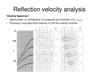
6. For multiple layers, t2 = t2(0) + x2/vrms2, so plots of t2vs x2 will give a straight line with slope of 1/vrms. • The root-mean square velocity (vrms) is determined by eq. 3.4 in terms of the interval velocity (vi) and travel time (Δti) of each layer interval (i). (Figs. 3.9 to 3-11)

8. For “real” data, we expect moveout of reflectors to decrease with depth (=time) as velocity increases with depth due to compaction

9. Various definitions of velocity (Box6.4) • Notice difference between vrms and vav but it is small • Note also that vnmo= vrmsonly for the small offset (spread) approximation (Fig. 3-22). For larger spread offsets, the best fit to flatten the actual moveout is not the same.

10. For continuous data (not individual picks) we need to flatten arrivals (ie remove increase in t as function of x and v) by stretching the time axis. This results in non-linear expansion of the time axis, which is greater for larger x and smaller v. This changes the frequency of the arrivals. (Fig. 3-13 and Table 3-2). When this effect becomes too large (generally in the upper 1-2 sec TWTT), we need to mute the result (Fig. 3-12). This can be done automatically for stretching greater than a certain amount, or by picking the front mutes by hand as we did to remove the refraction arrivals. (Fig. 3-14).

12. Methods for Velocity Analysis

13. Synthetic example with 4 layers showing CMP gather, velocity spectrum and t2-x2 plots. Spectrum is unnormalized, cross-correlation sum with a gated row plot.

14. Real example with 4 primary layers and multiple secondary layers. Spectrum is unnormalized, cross-correlation sum with contour plot.

15. Use of constant-velocity gathers (CVG) for a single CMP gather at various velocities to help detail exact nature of stacking velocities

17. Use of constant velocity stack (CVS) for range of gathers at different stacking velocities. Helpful in sections of low signal-to-noise (e.g. at greater depths in the section)

18. Limitations in accuracy and resolution of velocity estimates

19. Synthetic examples of 4 layers showing various plots of velocity spectra. Effect of spread (offset) length

20. Lack of long offsets reduce resolution of lower (high velocity) layers with smaller moveout

21. Lack of near-offsets reduce resolution of shallow layers Partial stacking (using incomplete fold) can save money (computer time) but can result in reduced resolution

22. Reduced resolution caused by decrease in signal-to-noise

24. Effect of dipping layer

25. Effect of dip is only significant when dip angle is large (i.e. > 20o)