Download

1 / 15
260 likes | 715 Views
INTERNATIONAL PHD PROJECTS IN APPLIED NUCLEAR PHYSICS AND INNOVATIVE TECHNOLOGIES This project is supported by the Foundation for Polish Science – MPD program, co-financed by the European Union within the European Regional Development Fund. Feynman Diagrams of the Standard Model.

E N D
INTERNATIONAL PHD PROJECTS IN APPLIED NUCLEAR PHYSICS AND INNOVATIVE TECHNOLOGIES This project is supported by the Foundation for Polish Science – MPD program, co-financed by the European Union within the European Regional Development Fund Feynman Diagrams of the Standard Model SedighehJowzaee PhD Seminar, 25 July 2013
Outlook • Introduction to the standard model • Basic information • Feynman diagram • Feynman rules • Feynman element factors • Feynman amplitude • Examples
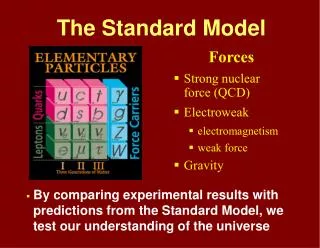
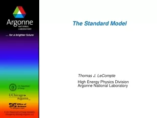
The Standard Model • The Standard Model of particles is a theory concerning the electromagnetic, weak and strong nuclear interactions • Collaborative effort of scientists around the world • Glashow's electroweak theory in 1960, Weinberg and Salam effort for Higgs mechanism in 1967 • Formulated in the 1970s • Incomplete theory • Does not incorporate the full theory of gravitation or predict the accelerating expansion of the universe • Does not contain any viable dark matter particle • Does not account neutrino oscillations and their non-zero masses
The Standard Model Gauge bosons Higgs bosons Generations of matter • The standard model has 61 elementary particles • The common material of the present universe is the stable particles, e, u, d
Gauge Bosons • Force carriers that mediate the strong, weak and electromagnetic fundamental interactions • Photons: mediate the electromagnetic force between charged particles • W, Z: mediate the weak interactions between particles of different flavors (quarks & leptons) • Gluons: mediate the strong interactions between color charged quarks • Forces are resulting from matter particles exchanging force mediating particles • Feynman diagram calculations are a graphical representation of the perturbation theory approximation, invoke “force mediating particles”
Feynman diagram • Schematic representation of the behavior of subatomic particles interactions • Nobel prize-winning American physicist Richard Feynman, 1948 • A Feynman diagram is a representation of quantum field theory processes in terms of particle paths • Feynman gave a prescription for calculation the transition amplitude or matrix elements from a field theory Lagrangian • |M|2 is the Feynman invariant amplitude • Transition amplitudes (matrix elements) must be summed over indistinguishable initial and final states and different order of perturbation theory
What do we study? • Reactions (A+BC+D+…) • Experimental observables: Cross sections, Decay width, scattering angles etc… • Calculation of or based on Fermi’s Golden rule: • _ decay rates (12+3+…+n) • _ cross sections (1+23+4+…+n) • Calculation of observable quantity consists of two steps: • 1. Determination of |M|2 we use the method of Feynman diagrams • 2. Integration over the Lorentz invariant phase space
Feynman rules time • 3 different types of lines: • Incoming lines: extend from the past to a vertex and represents an initial state • Outgoing lines: extend from a vertex to the future and represent the final state • (Incoming and outgoing lines carry an energy, momentum and spin) • Internal lines connect 2 vertices (a point where lines connect to another lines is an interaction vertex) • Quantum numbers are conserved in each vertex • e.g. electric charge, lepton number, energy, momentum • Particle going forwards in time, antiparticle backward in time • Intermediate particles are “virtual” and are called propagators • “Virtual” Particles do not conserve E, p • for ’s: E2-p20 • At each vertex there is a coupling constant • In all cases only standard model vertices allowed space time space • They are purely symbolic! Horizontal dimension is time but the other dimension DOES NOT represent particle trajectories!
Feynman interactions from the standard model • Because gluons carry color charge, there are three-gluon and four-gluon vertices as well as quark-quark-gluon vertices.
We construct all possible diagrams with fixed outer particles Example: for scattering of 2 scalar particles: • Since each vertex corresponds to one interaction Lagrangian term in the S matrix, diagrams with loops correspond to higher orders of perturbation theory • We classify diagrams by the order of the coupling constant (this is just perturbation Theory!!) • For a given order of the coupling constant there can be many diagrams • Must add/subtract diagram together to get the total amplitude, total amplitude must reflect the symmetry of the process • e+e- identical bosons in final state, amplitude symmetric under exchange of , : M=M1+M2 • Moller scattering: ei1-ei2-ef1-ef2- identical fermions in initial and final state, amplitude anti-symmetric under exchange of (i1,i2) and (f1,f2) : M=M1-M2 1/2 1/2 Tree diagram 1/2 1/2 1/2 1/2 2nd order perturbation 1st order perturbation 4th order perturbation 1/2
Feynman diagram element factors • Associate factors with elements of the Feynman diagram to write down the amplitude • The vertex factor (Coupling constant) is just the i times the interaction term in the momentum space Lagrangian with all fields removed • The internal line factor (propagator) is i times the inverse of kinetic operator (by free equation of motion) in the momentum space • Spin 0 : scalar field (Higgs, pions ,…) • Spin ½: Dirac field (electrons, quarks, leptons) scalar propagator multiplies by the polarization sum • Spin 1: Vector field • Massive (W, Z weak bosons) • Massless (photons) • External lines are represented by the appropriate polarization vector or spinor e.g. Fermions (ingoing,outgoing) u, ū ; antifermion ; photon em, em* ; scalar 1, 1
Feynman rules to extract M 1- Label all incoming/outgoing 4-momenta p1, p2,…, pn; Label internal 4-momenta q1,q2…,qn. 2- Write Coupling constant for each vertex 3- Write Propagator factor for each internal line 4- write E/p conservation for each vertex (2)44(k1+k2+k3); k’s are the 4-momenta at the vertex (+/– if incoming/outgoing) 5- Integration over internal momenta: add 1/(2)4d4q for each internal line and integrate over all internal momenta 6- Cancel the overall Delta function that is left: (2)44(p1+p2–p3…–pn) What remains is:
First order process • Simple example: F4-theory • We have just one scalar field and one vertex • We will work only to the lowest order momentum space momentum space The tree-level contribution to the scalar-scalar scattering amplitude in this F4-theory
Second order processes in QED • There is only one tree-level diagram