Download
1 / 25
250 likes | 337 Views
An overview of improvements in polarization analysis techniques from three years of WMAP observations, including foreground removal, data combination, and null tests.

E N D
Three-Year WMAP Observations: Polarization Analysis Eiichiro Komatsu The University of Texas at Austin Irvine, March 23, 2006
First Year (TE) Foreground Removal Done in harmonic space Null Tests Only TB Data Combination Ka, Q, V, W are used Data Weighting Diagonal weighting Likelihood Form Gaussian for Cl Cl estimated by MASTER Three Years (TE,EE,BB) Foreground Removal Done in pixel space Null Tests Year Difference & TB, EB, BB Data Combination Only Q and V are used Data Weighting Optimal weighting (C-1) Likelihood Form Gaussian for the pixel data Cl not used at l<23 Summary of Improvements in the Polarization Analysis These are improvements only in the analysis techniques: there are also various improvements in the polarization map-making algorithm. See Jarosik et al. (2006)
K Band (23 GHz) Dominated by synchrotron; Note that polarization direction is perpendicular to the magnetic field lines.
Ka Band (33 GHz) Synchrotron decreases as n-3.2 from K to Ka band.
Q Band (41 GHz) We still see significant polarized synchrotron in Q.
V Band (61 GHz) The polarized foreground emission is also smallest in V band. We can also see that noise is larger on the ecliptic plane.
W Band (94 GHz) While synchrotron is the smallest in W, polarized dust (hard to see by eyes) may contaminate in W band more than in V band.
Polarization Mask (P06) • Mask was created using • K band polarization intensity • MEM dust intensity map fsky=0.743
Masking Is Not Enough: Foreground Must Be Cleaned • Outside P06 • EE (solid) • BB (dashed) • Black lines • Theory EE • tau=0.09 • Theory BB • r=0.3 • Frequency = Geometric mean of two frequencies used to compute Cl Rough fit to BB FG in 60GHz
Template-based FG Removal • The first year analysis (TE) • We cleaned synchrotron foreground using the K-band correlation function (also power spectrum) information. • It worked reasonably well for TE (polarized foreground is not correlated with CMB temperature); however, this approach is bound to fail for EE or BB. • The three year analysis (TE, EE, BB) • We used the K band polarization map to model the polarization foreground from synchrotron in pixel space. • The K band map was fitted to each of the Ka, Q, V, and W maps, to find the best-fit coefficient. The best-fit map was then subtracted from each map. • We also used the polarized dust template map based on the stellar polarization data to subtract the dust contamination. • We found evidence that W band data is contaminated by polarized dust, but dust polarization is unimportant in the other bands. • We don’t use W band for the three year analysis (for other reasons).
It Works Well!! • Only two-parameter fit! • Dramatic improvement in chi-squared. • The cleaned Q and V maps have the reduced chi-squared of ~1.02 per DOF=4534 (outside P06)
3-sigma detection of EE. The “Gold” multipoles: l=3,4,5,6. BB consistent with zero after FG removal.
Residual FG unlikely in Q&V • Black: EE • Blue: BB • Thick: 3-year data coadded • Thin: year-year differences • Red line: upper bound on the residual synchrotron • Brown line: upper bound on the residual dust • Horizontal Dotted: best-fit CMB EE (tau=0.09)
Null Tests • It’s very powerful to have three years of data. • Year-year differences must be consistent with zero signal. • yr1-yr2, yr2-yr3, and yr3-yr1 • We could not do this null test for the first year data. • We are confident that we understand polarization noise to a couple of percent level. • Statistical isotropy • TB and EB must be consistent with zero. • Inflation prior… • We don’t expect 3-yr data to detect any BB.
Data Combination (l<23) • We used Ka, Q, V, and W for the 1-yr TE analysis. • We use only Q and V for the 3-yr polarization analysis. • Despite the fact that all of the year-year differences at all frequencies have passed the null tests, the 3-yr combined power spectrum in W band shows some anomalies. • EE at l=7 is too high. We have not identified the source of this anomalous signal. (FG is unlikely.) • We have decided not to use W for the 3-yr analysis. • The residual synchrotron FG is still a worry in Ka. • We have decided not to use Ka for the 3-yr analysis. • KaQVW is ~1.5 times more sensitive to tau than QV. • Therefore, the error reduction in tau by going from the first-year (KaQVW) to three-year analysis (QV) is not as significant as one might think from naïve extrapolation of the first-year result. • There is also another reason why the three-year error is larger (and more accurate) – next slide.
Correlated Noise • At low l, noise is not white. • 1/f noise increases noise at low l • See W4 in particular. • Scan pattern selectively amplifies the EE and BB spectra at particular multipoles. • The multipoles and amplitude of noise amplification depend on the beam separation, which is different from DA to DA. Red: white noise model (used in the first-year analysis) Black: correlated noise model (3-yr model)
Low-l TE Data: Comparison between 1-yr and 3-yr • 1-yr TE and 3-yr TE have about the same error-bars. • 1yr used KaQVW and white noise model • Errors significantly underestimated. • Potentially incomplete FG subtraction. • 3yr used QV and correlated noise model • Only 2-sigma detection of low-l TE.
High-l TE Data • The amplitude and phases of high-l TE data agree very well with the prediction from TT data and linear perturbation theory and adiabatic initial conditions. (Left Panel: Blue=1yr, Black=3yr) Amplitude Phase Shift
High-l EE Data • When QVW are coadded, the high-l EE amplitude relative to the prediction from the best-fit cosmology is 0.95 +- 0.35. • Expect ~4-5sigma detection from 6-yr data. WMAP: QVW combined
Optimal Analysis of the Low-l Polarization Data • In the likelihood code, we use the TE power spectrum data at 23<l<500, assuming that the distribution of high-l TE power spectrum is a Gaussian. • An excellent approximation at high multipoles. • This part is the same as the first-year analysis. • However, we do not use the TE, EE or BB power spectrum data at l<23 in the likelihood code. • In fact, we do not use the EE or BB power spectrum data anywhere in the likelihood code. • The distribution of power spectrum at low multipoles is highly non-Gaussian. • We use the pixel-based exact likelihood analysis, using the fact that the pixel data (both signal and noise) are Gaussian.
Exact TE,EE,BB Likelihood Gaussian Likelihood for T, Q, U T Factorized… By Rotating the Basis.
Stand-alone t • Tau is almost entirely determined by the EE data. • TE adds very little. • Black Solid: TE+EE • Cyan: EE only • Dashed: Gaussian Cl • Dotted: TE+EE from KaQVW • Shaded: Kogut et al.’s stand-alone tau analysis from Cl TE • Grey lines: 1-yr full analysis (Spergel et al. 2003)
Tau is Constrained by EE • The stand-alone analysis of EE data gives • tau = 0.100 +- 0.029 • The stand-alone analysis of TE+EE gives • tau = 0.092 +- 0.029 • The full 6-parameter analysis gives • tau = 0.093 +- 0.029 (Spergel et al.; no SZ) • This indicates that the stand-alone EE analysis has exhausted most of the information on tau contained in the polarization data. • This is a very powerful statement: this immediately implies that the 3-yr polarization data essentially fixes tau independent of the other parameters, and thus can break massive degeneracies between tau and the other parameters. (Rachel Bean’s talk)
Stand-alone r • Our ability to constrain the amplitude of gravity waves is still coming mostly from TT. • BB information adds very little. • EE data (which fix the value of tau) are also important, as r is degenerate with the tilt, which is also degenerate with tau.
Summary • Understanding of • Noise, • Systematics, • Foreground, and • Analysis techniques such as • Exact likelihood method • have significantly improved from the first-year release. • Tau=0.09+-0.03 • To-do list for the next data release(!) • Understand W band better • Understand foreground in Ka better • These improvements, combined with more years of data, would further reduce the error on tau. • 3-yr KaQVW combination gave delta(tau)~0.02 • 6-yr KaQVW would give delta(tau)~0.014 (hopefully)