summary
summary. Two-sided t-test . difference between means, i.e. variability between samples. variability within samples. This is not an exact formula! It just demonstrates main ingrediences. Two-sided t-test . The numerator indicates how much the means differ.


summary
E N D
Presentation Transcript
Two-sided t-test difference between means, i.e. variability between samples variability within samples This is not an exact formula! It just demonstrates main ingrediences.
Two-sided t-test • The numerator indicates how much the means differ. • This is an explained variation because it most likely results from the differences due to the treatment or just dut to the differences in the populations (recall beer prices, different brands are differently exppensive). • The denominator is a measure of an error. It measures individual differences of subjects. • This is considered anerror variation because we don't know why individual subjects in the same group are different.
ANOVA • Compare as many means as you want just with one test.
Total variability • What is the total number of degrees of freedom? • Likewise, we have a total variation
Hypothesis • Let's compare three samples with ANOVA. Just try tu guess what the hypothesis will be? at least one pair of samples is significantly different • Follow-up multiple comparison steps – see which means are different from each other.
Multiple comparisons problem • And there is another (more serious problem) with many t-tests. It is called a multiple comparisons problem. http://www.graphpad.com/guides/prism/6/statistics/index.htm?beware_of_multiple_comparisons.htm
Post hoc tests • F-test in ANOVA is the so-called omnibus test. It tests the means globally. It says nothing about which particular means are different. • post hoc tests, multiple comparison tests. • Tukey Honestly Significant Differences TukeyHSD(fit) # where fit comes from aov()
ANOVA assumptions • normality – all populations samples come from are normal • homogeneity of variance – variances are equal • independence of observations – the results found in one sample won't affect others • Most influencial is the independence assumption. Otherwise, ANOVA is relatively robust. • We can sometimes violate • normality – large sample size • variance homogeneity – equal sample sizes + the ratio of any two variances does not exceed four
ANOVA kinds • one-way ANOVA (analýza rozptylu při jednoduchém třídění, jednofaktorová ANOVA) aov(beer_brands$Price~beer_brands$Brand) • two-way ANOVA (analýza rozptylu dvojného třídění, dvoufaktorová ANOVA) • Example: engagement ratio, measure two educational methods (with and without song) for men and women independently • aov(engagement~method+sex) • interactions between factors dependent variable independent variable
Introduction • Up to this point we've been working with only one variable. • Now we are going to focus on two variables. • Two variables that are probably related. Can you think of some examples? • weight and height • time spent studying and your grade • temperature outside and ankle injuries
Car data • x – predictor, explanatory, independent variable • How do you think y is called? Think about opposites to x name. • outcome • determiner • response • stand-alone • dependent
Car data • How may we show these variables have a relationship? • Tell me some of yours ideas. • scatterplot
Correlation • Relation between two variables = correlation • strong relationship = strong correlation, high correlation Match these strong positive strong negative weak positive weak negative
Correlation coefficient • r (Pearson's r) - a number that quantifies the relationship. • … covariance of X and Y. A statistic for how much X and Y co-vary. In other words, how much do they vary together. • … standard deviations of X and Y. Describes, how to variables vary apart from each other, rather than with each other. • measures the strength of the relationship by looking at how closely the data falls along a straight line.
Covariance • Watch explanation video. http://www.youtube.com/watch?v=35NWFr53cgA divide by n-1 for sample but by n for population
Coefficient of determination • Coefficient of determination - is the percentage of variation in Y explained by the variation in X. • Percentage of variance in one variable that is accounted for by the variance in the other variable. r2 = 0 r2 = 0.25 r2 = 0.81 from http://www.sagepub.com/upm-data/11894_Chapter_5.pdf
+1 +0.14 +0.93 -1 -0.73
If X is age in years and Y age in months, what will the correlation coefficient be? • +1.0 • X is hours you're awake a day, Y is hours you're asleep a day. • -1.0
Crickets • Find a cricket, count the number of its chirps in 15 seconds, add 37, you have just approximated the outside temperature in degrees Fahrenheit. • National Service Weather Forecast Office: http://www.srh.noaa.gov/epz/?n=wxcalc_cricketconvert
Hypothesis testing • Even when two variables describing a sample of data may seem they have an relationship, this could just be due to the chance. The situation in population may be different. • … sample corr. coeff., … population corr. coeff. • How hypotheses will look like? A B C D
Hypothesis testing • test statistic has a t-distribution • Example: we are measuring relationship between two variables, we have 25 participants, we get the t-statistic = 2.71. Is there a significant relationship between X and Y? • , non-directonal test,
Confidence intervals • reject the null • fail to reject the null 95% CI = (-0.3995, 0.0914) 95% CI = 0.1369, 0.5733) try to guess: • reject the null • fail to reject the null Statistics course from https://www.udacity.com
Hypothesis testing • A statiscally correct way how to decide about the relationship between two variables is, of course, hypothesis testing. • In these two particular cases:
Correlation vs. causation • causation – one variable causes another to happen • e.g. the facts it is raining cause people to take their umbrellas to work • correlation – just means there is a relationship • e.g. do happy people have more friends? Are they just happy because they have more friends? Or they act a certain way which causes them to have more friends.
Correlation vs. causation • There is a strong relationship between the ice cream consumption and the crime rate. • How could this be true? • The two variables must have something in common with one another. It must be something that relates to both level of ice cream consumption and level of crime rate. Can you guess what that is? • Outside temperature. from causeweb.org
Correlation vs. causation • If you stop selling ice cream, does the crime rate drop? What do you think? • That’s because of the simple principle that correlations express the association that exists between two or more variables; they have nothing to do with causality. • In other words, just because level of ice cream consumption and crime rate increase/descrease together does not mean that a change in one necessarily results in a change in the other. • You can’t interpret associations as being causal.
Correlation vs. causation • In an ice cream example, there exist a variable (outside temperature) we did not realize to control. • Such variable is called third variable, confounding variable, lurking variable. • The methodologies of scientific studies therefore need to control for these factors to avoid a 'false positive‘ conclusion that the dependent variables are in a causal relationship with the independent variable. • Let’s have a look at dependence of murder rate on temperature.
from http://www-personal.umich.edu/~bbushman/BWA05a.pdf Journal of Personality and Social Psychology, 2005, Vol. 89, No. 1, 62–66
high assault period low assault period from http://www-personal.umich.edu/~bbushman/BWA05a.pdf Journal of Personality and Social Psychology, 2005, Vol. 89, No. 1, 62–66
Correlation and regression analysis • Correlation analysis investigates the relationships between variables using graphs or correlation coefficients. • Regression analysis answers the questions like: which relationship exists between variables X and Y (linear, quadratic ,….), is it possible to predict Y using X, and with what error?
Simple linear regression • also single linear regression (jednoduchá lineární regrese) • one y(dependent variable, závisle proměnná), one x (independent variable, nezávisle proměnná) • – y-intercept (constant), – slope • is estimated value, so to distinguish it from the actual value corresponding to the given statisticans use
Data set • Students in higher grades carry more textbooks. • Weight of the textbooks depends on the weight of the student.
strong positive correlation, r = 0.926 outlier from Intermediate Statistics for Dummies
Build a model • Find a straight line y = a + bx
Interpretation • y-intercept (3.69 in our case) • it may or may not have a practical meaning • Does it fall within actual values in the data set? If yes, it is a clue it may have a practical meaning. • Does it fall within negative territory where negative y-value are not possible? (e.g. weights can’t be negative) • Does a value x = 0 have practical meaning (student weighting 0)? • However, even if it has no meaning, it may be necessary (i.e. significantly different from zero)! • slope • change in y due to one-unit increase in x (i.e. if student’s weight increases by 1 pound, its textbook’s weight increases by 0.113 pounds) • now you can use regression line to estimate y value for new x
Regression model conditions • After building a regression mode you need to check if the required conditions are met. • What are these conditions? • The y’s have to have normal distribution for each value of x. • The y’s have to have constant spread (standard deviation) for each value of x.
Normal y’s for every x • For any value of x, the population of possible y-values must have a normal distribution. from Intermediate Statistics for Dummies
Homoscedasticity condition As you move from left to the right on the x-axis, the spread around y-values remain the same. source: wikipedia.org
Confidence and prediction limit 95% confidence limits – this interval includes the true regression line with 95% probability. (pás spolehlivosti) 95% prediction limits – this interval represents the 95% probability for the values of the dependent variable. i.e. 95% of data points lie within these lines. (pás predikce)
Residuals • To check the normality of y-values you need to measure how far off your predictions were from the actual data, and to explore these errors. • residual(residuum, reziduální hodnota predikce)