Chapter 5 The Simplex Method
Chapter 5 The Simplex Method. The most popular method for solving Linear Programming Problems We shall present it as an Algorithm. General Structure of Algorithms. Initialise. Check for desired results. Yes. Stop. Iterate. No. Perform a sequence of repetitive steps.

Chapter 5 The Simplex Method
E N D
Presentation Transcript
Chapter 5The Simplex Method The most popular method for solving Linear Programming Problems We shall present it as an Algorithm
General Structure of Algorithms Initialise Check for desired results Yes Stop Iterate No Perform a sequence of repetitive steps
Construct a feasible extreme point Is this point optimal ? Yes Stop Iterate No Move along an edge to a better extreme point
Missing Details • Initialisation: • How do we represent a feasible extreme point algebraically? • Optimality Test: • How do we determine whether a given extreme point is optimal? • Iteration: • How do we move a long an edge to a better adjacent extreme point?
5.1 initialisation • Transform the LP problem given in a standardform into a canonical form. • This involves the introduction of slackvariables, one for each functional constraint. • Thus if we start with n variables and m functional constraints, we end up with n+m variables and m functional equality constraints.
Standard Form • opt=max • ~ • bi ≥ 0 , for all i.
Observation • The i-th slack variable measure the “distance” of the point x=(x1,...,xn) from the hyperplanedefining the i-th constraint (This is not a Euclidean distance). • Thus, if the i-th slack variable is equal to zerothe point x= (x1,...,xn) is on the i-th hyperplane. Otherwise it is not. • The original variables “measure” the distance to the hyperplanes defining the respective non-negativityconstraints.
Example x3,x4,x5 are slack variables
Why do we do this? If we use the slack variables as a basis, we obtain a feasible extreme point !!!
5.5.1 Definition A basic feasible solution is a basic solution that satisfies the non-negativity constraint. Observation: A basic feasible solution is an extreme point of the feasible region. Thus: Initialisation involves constructing a basicfeasible solution using the slack varaibles.
Example Initialbasic feasible solution: x =(0,0,40,30,15), namely x1 = 0 x2 = 0 x3 = 40 x4 = 30 x5 =15 x3,x4,x5 are slack variables
Summary of the Initialisation Step • Select the slack variables as basic • Comments: • Simple • Not necessarily good selection: the first basic feasible solution can be (very) far from the optimal solution.

