Simplex Method
Simplex Method . Solution of a Minimization Problem. Simplex Solution of a Minimization Problem. - Linear programming minimization model . minimize Z = 6x 1 + 3x 2 subject to 2x 1 + 4x 2 16

Simplex Method
E N D
Presentation Transcript
Simplex Method Solution of a Minimization Problem
Simplex Solution of a Minimization Problem - Linear programming minimization model. minimize Z = 6x1+ 3x2 subject to 2x1 + 4x216 4x1 + 3x224 x1, x2 0
Simplex Solution of a Minimization Problem - Model is trans formed into standard form by subtracting surplus variables: minimize Z = 6x1 + 3x2 + 0s1 + 0s2 subject to 2x1 + 4x2 - s1= 16 4x1 + 3x2 - s2= 24 x1, x2, s1, s2 0
Simplex Solution of a Minimization Problem - However, transforming a model into standard form by subtracting surplus variables will not work in the simplex method. Graph of the fertilizer example
Simplex Solution of a Minimization Problem - An artificial variable allows for an initial basic feasible solution at the origin, but it has no real meaning. - Artificial variables are assigned a large cost in the objective function to eliminate them from the final solution: minimize Z = 6x1+ 3x2 + 0s1 + 0s2 + MA1 + MA2 subject to 2x1 + 4x2 - s1 + A1= 16 4x1 + 3x2 - s2+ A2= 24 x1, x2, s1, s2 , A1, A2 0
Simplex Solution of a Minimization Problem - The cj - zj row is changed to zj - cj in the simplex tableau for minimization problems. - Artificial variables are always included as part of the initial basic feasible solution when they exist. The Initial Simplex Tableau
Simplex Solution of a Minimization Problem - The second simplex tableau is developed using the simplex formulas presented earlier. - Once an artificial variable is selected as the leaving variable, it will never reenter the tableau, so it can be eliminated. The Second Simplex Tableau
Simplex Solution of a Minimization Problem - The third simplex tableau , with x1 replacing A2. The Third Simplex Tableau
Simplex Adjustments for a Minimization Problem 1. Transform all constraints to equations by subtracting a surplus varible and adding an artificial variable. 2. Assign a cj value of M to each artificial variable in the objective function. 3. Change the cj -zj row to zj - cj.
A Mixed Constraint Problem - A mixed constraint problem includes a combination of and constraints. - Example problem: maximize Z = 400x1+ 200x2 subject to x1 + x2 = 30 2x1 + 8x2 80 x1 20 x1, x20
A Mixed Constraint Problem - An artificial variable is added to an equality (=) constraint for standard form - An artificial variable in a maximization problem is given a large cost contribution to drive it out of the problem. - The transformed linear programming problem: maximize Z = 400x1+ 200x2 + 0s1 + 0s2 - MA1 - MA2 subject to x1 + x2 + A1= 30 2x1 + 8x2 - S1 + A2= 80 x1 + s2= 20 x1, x2, s1, s2, A1, A2 0
A Mixed Constraint Problem The Initial Simplex Tableau
A Mixed Constraint Problem The Second Simplex Tableau
A Mixed Constraint Problem The Third Simplex Tableau
A Mixed Constraint Problem - Summary of rules for transforming all three types of model constraints.
Irregular Types of Linear Programming Problems • Problems with more than one solution • Infeasible problems • Problems with unbounded solutions • Problems with ties for the pivot column • Problems with ties for the pivot row • Problems with constraints with negative quantity values
Multiple Optimal Solutions - Alternate optimal solutions have the same Z value but different variable values. - Beaver Creek Pottery Company problem changed as follows: maximize Z = $40x1 + 30x2 subject to x1 + 2x2 40 (labor, hours) 4x1 + 3x2 120 (clay, pounds) x1, x2 0 Graph of the Beaver Creek Pottery Company example with multiple optimal solutions
Multiple Optimal Solutions - Optimal simplex tableau shown below; corresponds to point C in the Figure - For a multiple optimal solution the cj - zj (or zj - cj) value for a nonbasic variable in the final tableau equals zero. The Optimal Simplex Tableau
Multiple Optimal Solutions - Alternate solution shown below; corresponds to point B in Figure 5. - An alternate optimal solution is determined by selecting the nonbasic variable with cj - zj = 0 as the entering variable. The Alternative Optimal Tableau
An Infeasible Problem - An infeasible problem does not have a feasible solution space. - Example: maximize Z = 5x1 + 3x2 subject to 4x1 + 2x2 8 x1 4 x2 6 x1, x2 0 Graph of an infeasible problem
An Infeasible Problem - An infeasible problem has an artificial variable in the final simplex tableau. The Final Simplex Tableau for an Infeasible Problem
An Unbounded Problem - In an unbounded problem the objective function can increase indefinitely because the solution space is not closed. - Example: maximize Z = 4x1 + 2x2 subject to x1 4 x2 2 x1, x2 0 An unbounded problem
An Unbounded Problem - A pivot row cannot be selected for an unbounded problem - An unbounded solution, like an infeasible solution, reflects an error in defining the problem or in formulating the model. The Second Simplex Tableau
Tie for the Pivot Column/Pivot Row - A tie for the pivot column is broken arbitrarily. - A tie for the pivot row is broken arbitrarily and can lead to degeneracy. - Degeneracy occurs when it is possible for subsequent simplex tableau solutions to degenerate so that the objective function value never improves and optimality never results. maximize Z = 4x1 + 6x2 subject to 6x1+ 4x2 24 x2 3 5x1 + 10x2 40 x1, x2 0 The Second Simplex Tableau with a Tie for the Pivot Row
Tie for the Pivot Column/Pivot Row - A quantity value of zero now appears in the s1 row, representing the degenerate condition resulting from the tie for the pivot row. The Third Simplex Tableau with Degeneracy
Tie for the Pivot Column/Pivot Row - The optimal solution did not change from the third to the optimal tableau. The Optimal Simplex Tableau for a Degenerate Problem
Tie for the Pivot Column/Pivot Row - Degeneracy occurs in a simplex problem when a problem continually loops back to the same solution or tableau. Graph of a degenerate solution
Negative Quantity Values - Standard form for simplex solution requires positive right-hand- side values. - A negative right-hand-side value is changed to a positive by multiplying the constraint by -1, which changes the inequality sign: -6x1 + 2x2 -30 (-1)(-6x1 + 2x2 -30) 6x1 - 2x2 30
Summary Simplex Adjustments for a Minimization Problem 1. Transform all constraints to equations by subtracting a surplus variable and adding an artificial variable. 2. Assign a cj value of M to each artificial variable in the objective function. 3. Change the cj -zj row to zj - cj. A Mixed Constraint Problem
Summary By using the Simplex Method : • Alternative Optimum • Unbounded Solution • Infeasible Solution