Simulating Multivariate Random Normal Data Using Statistical Computing Platform R
Many faculty members, as well as students, in the area of educational research methodology, sometimes have a need for generating data to use for simulation and computation purposes, demonstration of multivariate analysis techniques, or construction of student projects or assignments. As a great teaching tool, using simulated data helps us understand the intricacies of statistical concepts and techniques. The process of generating multivariate normal data is a nontrivial process and practical guides without dense mathematics are limited in the literature Nissen and Saft, 2014 . Hence, the purpose of this paper is to offer researchers a practical guide for and a quick access to generating multivariate random data with a given mean and variance covariance structure. A detailed outline of simulating multivariate normal data with a given mean and variance covariance matrix using Eigen or spectral and Cholesky decompositions is presented and implemented in statistical computing platform R version 3.4.4 R Core Team, 2018 . Mehmet Turegun "Simulating Multivariate Random Normal Data using Statistical Computing Platform R" Published in International Journal of Trend in Scientific Research and Development (ijtsrd), ISSN: 2456-6470, Volume-3 | Issue-4 , June 2019, URL: https://www.ijtsrd.com/papers/ijtsrd23987.pdf Paper URL: https://www.ijtsrd.com/humanities-and-the-arts/education/23987/simulating-multivariate-random-normal-data-using-statistical-computing-platform-r/mehmet-turegun<br>

Simulating Multivariate Random Normal Data Using Statistical Computing Platform R
E N D
Presentation Transcript
International Journal of Trend in Scientific Research and Development (IJTSRD) Volume: 3 | Issue: 4 | May-Jun 2019 Available Online: www.ijtsrd.com e-ISSN: 2456 - 6470 Simulating Multivariate Random Normal Data using Statistical Computing Platform R Mehmet Turegun Professor, Barry University, Miami Shores, Florida How to cite this paper:Mehmet Turegun "Simulating Random Normal Data using Statistical Computing Platform R" Published in International Journal of Trend in Scientific Research and Development (ijtsrd), ISSN: 2456- 6470, Volume-3 | Issue-4, June 2019, pp.1126-1132, URL: https://www.ijtsrd.c om/papers/ijtsrd23 987.pdf Copyright © 2019 by author(s) and International Journal of Trend in Scientific Research and Development Journal. This is an Open Access article distributed under the terms of the Creative Commons Attribution License (CC BY 4.0) (http://creativecommons.org/licenses/ by/4.0) Although some of these techniques are robust to the violation of the multivariate normality assumption, such violations of multivariate normality increase the chances of researchers committing to Type I and/or Type II errors. Additionally, the correlations among variables can be distorted as a result of non-normality (Courtney and Chang, 2018). Hence, a major portion of the data screening efforts for our statistical analyses needs to focus on assessing and correcting for non-normality. However, in many cases it can be better to provide our audiences with a multivariate normal data set in order for them to understand what such data look like before they can try to assess or identify non-normality. Furthermore, many teachers may recall instances in which they wished that they had a multivariate raw dat set with a specified set of means, standard deviations and correlation matrix for the variables. It is for these reasons, a brief discussion and an accessible illustration of how to simulate multivariate normal data with a given mean and variance-covariance matrix using Eigen and Cholesky decompositions may be a necessary topic. Generating Multivariate Normal Data Although there are several studies reporting the generation of multivariate normal data using various software packages and computing platforms, the process of generating multivariate normal data is a nontrivial process and practical guides without dense mathematics are limited in the ABSTRACT Many faculty members, as well as students, in the area of educational research methodology, sometimes have a need for generating data to use for simulation and computation purposes, demonstration of multivariate analysis techniques, or construction of student projects or assignments. As a great teaching tool, using simulated data helps us understand the intricacies of statistical concepts and techniques. The process of generating multivariate normal data is a nontrivial process and practical guides without dense mathematics are limited in the literature (Nissen and Saft, 2014). Hence, the purpose of this paper is to offer researchers a practical guide for and a quick access to generating multivariate random data with a given mean and variance-covariance structure. A detailed outline of simulating multivariate normal data with a given mean and variance- covariance matrix using Eigen (or spectral) and Cholesky decompositions is presented and implemented in statistical computing platform R version 3.4.4 (R Core Team, 2018). Keywords: Cholesky decomposition, Eigen decomposition, simulation of multivariate random normal data, variance-covariance matrix, R 1.INTRODUCTION Many of the multivariate statistical techniques, such as multiple regression and multiple analysis of variance, require an assumption of multivariate normality of the continuous variables. literature (Demirtas, 2004; Goldman and McKenzie, 2009; Hunt, 2001; Nissen and Saft, 2014). One can use several different ways to decompose a given data matrix. The two most widely used methods are the QR decomposition, which decomposes a matrix into an orthogonal matrix and an upper triangular matrix, and the singular value decomposition (SVD). There are also Cholesky and Eigen decompositions, which are special cases of the former two. The QR and the SVD are different from the Cholesky and Eigen decompositions because the latter approaches require the input data to be a square matrix, whereas QR and SVD can be applied to an m × n matrix. The Eigen and Cholesky decompositions are the two of the most commonly used methods. Although the Eigen value decomposition method is more stable, the Cholesky decomposition method is faster, but not by a considerable amount (Venables and Ripley, 2002). The statistical computing platform R version 3.4.4 (R Core Team, 2018) was used to implement the above mentioned decompositions to generate several multivariate random normal data sets. Eigen Decomposition In the Eigen decomposition approach, given a correlation matrix Σ, one can define a matrix V, which consists of the product of the eigenvectors of Σ, E, and the diagonal values of the square root of eigenvalues of Σ. One can then compute X= Multivariate IJTSRD23987 @ IJTSRD | Unique Paper ID - IJTSRD23987 | Volume – 3 | Issue – 4 | May-Jun 2019 Page: 1126
International Journal of Trend in Scientific Research and Development (IJTSRD) @ www.ijtsrd.com eISSN: 2456-6470 Z VT where the elements of Z is a random sample from a normal distribution with mean 0 and variance 1. The partial R script for generating the multivariate normal data for three variables and 5,000 cases is given in Figure 1. nobs=5000 nvars=3 corMat<-matrix(cbind(1,.2,.3,.2,1,.2,.3,.2,1),nrow=nvars) # Check to see if variance-covariance matrix is symmetric and positive definite det(corMat) min(eigen(corMat)$values) ev<-eigen(corMat) V<-ev$vectors%*%(diag(sqrt(ev$values))) t(V)%*%V Z<-matrix(rnorm(nobs*nvars),nrow=nobs,ncol=nvars) Xeigen<- Z%*%t(V) # Compare the simulated correlation matrix to the original correlation matrix cor(Xeigen) corMat # Calculate the residuals res<-round(corMat-cor(Xeigen),3) # Calculate the Root mean square residuals (RMSR) sqrt(sum(res^2)/(nvars*nvars)) # Means and SDs for the simulated data # Create the raw data dataeigen<-as.data.frame(Xeigen) names(dataeigen)<-c(“x1”,”x2”,”x3”) # Write raw data to a file and save Figure1. Partial R script for implementing the Eigen decomposition for generating multivariate normal data Cholesky Decomposition Alternatively, one can generate a multivariate normal random sample by using a matrix operation called Cholesky decomposition, which is considered to provide an efficient method for the case of a symmetric positive definite variance- covariance matrix Σ. The probability density function, pdf, of the multivariate normal distribution for the m dimensional vector X can be given by the following formula. pdf(X) = (2π*det(Σ))^(-m/2) * exp(-0.5*(X-MU)T*(Σ-1)*(X-MU)) In this equation, MU is the mean vector, and sigma, Σ, is a positive definite symmetric matrix called the variance-covariance matrix. To create X, an m x n matrix containing n samples from this distribution, it is only necessary to create an m x n vector Z, each of whose elements is a sample of the 1-dimensional normal distribution with mean 0 and variance 1. Then, one can proceed to determine the upper triangular Cholesky factor A of the matrix Σ, so that Σ = AT A. As a final step in the process, one needs to compute X = MU + AT Z. In order to simulate from a multivariate normal distribution with a mean μ vector and variance-covariance matrix Σ, one needs to be able to express the variance-covariance matrix as Σ=AAT for some matrix A. This is the case if and only if Σ is a positive semi-definite or positive definite matrix, which is a symmetric matrix with non-negative eigenvalues (Golub and Van Loan, 1996). The Cholesky decomposition of Σ yields a lower triangular matrix A such that A times its transpose, AT, gives Σ back again. This matrix is used in generating the multivariate random normal data in the following manner. If one generates a vector Z of standard random normal numbers having a length equal to the dimensions of A, then multiplying A, which is the Cholesky decomposition of Σ, by Z, and adding the desired mean, one ends up with a matrix of the desired random samples. Without the detailed mathematical proofs using matrix algebra, one can reason through this process conceptually by making the following observations. Var(AZ) = A Var(Z) AT as A is just a constant. Since the standard normal random numbers have a variance of 1, the variance of Z is the identity matrix I. Notice that Variance(AZ) = A I AT = A AT = Σ. Hence, the random data set generated aligns with the desired variance-covariance structure. The partial R script for generating the multivariate normal data for three variables and 5,000 cases is given in Figure 2. @ IJTSRD | Unique Paper ID - IJTSRD23987 | Volume – 3 | Issue – 4 | May-Jun 2019 Page: 1127
International Journal of Trend in Scientific Research and Development (IJTSRD) @ www.ijtsrd.com eISSN: 2456-6470 nobs=5000 nvars=3 corMat<-matrix(cbind(1,.2,.3,.2,1,.2,.3,.2,1),nrow=nvars) # Check to see if variance-covariance matrix is symmetric and positive definite det(corMat) min(eigen(corMat)$values) meanvec<-c(0,0,0) Z<-matrix(rnorm(nobs*nvars),nobs,nvars) X<- Z%*%chol(corMat)+t(matrix(rep(meanvec,nobs),nrow=nvars)) # Compare the simulated correlation matrix to the original correlation matrix cor(X) corMat # Calculate the residuals res<-round(corMat-cor(X),3) # Calculate the Root Mean Square Residuals (RMSR) sqrt(sum(res^2)/(nvars*nvars)) # Means and SDs for the simulated data # Create the raw data datachol<-as.data.frame(X) names(datachol)<-c(“x1”,”x2”,”x3”) # Write raw data to a file and save Figure2. Partial R script for implementing the Cholesky decomposition for generating multivariate normal data A comparison of the results of the multivariate normal data generated by using the Eigen and Cholesky decompositions is summarized in Table 1. Throughout the table, the comparisons are based on a multivariate normal data set generated for 5,000 observations and three variables, x1, x2, and x3. In addition to the theoretical and empirical means, standard deviations, correlation matrices, and residual correlation matrices, the root mean square error (RMSE) values, which are obtained by squaring the residuals, averaging the squares, and taking the square root, are also given in Table 1. The RMSE values for the multivariate random data generated by Eigen and Cholesky decompositions are both less than .05. Table1. Comparison of Eigen and Cholesky decompositions for generating multivariate normal data consisting three variables, x1, x2, and x3 for 5,000 observations Comparison Eigen Decomposition Cholesky Decomposition Theoretical means (.0, .0, .0) Empirical means (.010, .002, .006) Theoretical SDs (1.0, 1.0, 1.0) Empirical SDs (.993, 1.002, 1.000) Theoretical Correlation Matrices (.3,. 2, 1) Empirical Correlation Matrices (.275, .192, 1.000) Residual Correlation Matrices Root Mean Square Errors (RMSE) 0.017 Another comparison of the multivariate normal data generated by Eigen and Cholesky decompositions can be made based on the results of the multivariate normality tests for the simulated data. The multivariate normality test is based on the mvn() function of the R package MVN. The mvn() function uses the Mardia test for multivariate outlier detection and normality, which is tested based on skewness and kurtosis values. Additional univariate normality tests are conducted using the Anderson- Darling (A-D) test. Table 2 displays a summary of the results. (.0, .0, .0) (.020, -.005, .015) (1.0, 1.0, 1.0) (1.016, .9999, 1.015) (1, .2, .3) (.2, 1, .2) (.3,. 2, 1) (1.000, .195, .299) (.195, 1.000, .222) (.299, .222, 1.000) (.000, .005, .001) (.005, .000, -.022) (.001, -.022, .000) 0.011 (1, .2, .3) (.2, 1, .2) (1.000, .225, .275) (.225, 1.000, .192) (.000, -.025, .025) (-.025, .000, .008) (.025, .008, .000) @ IJTSRD | Unique Paper ID - IJTSRD23987 | Volume – 3 | Issue – 4 | May-Jun 2019 Page: 1128
International Journal of Trend in Scientific Research and Development (IJTSRD) @ www.ijtsrd.com eISSN: 2456-6470 Table2. Comparison of the descriptive statistics, univariate and multivariate normality tests for the data generated by using Eigen and Cholesky decompositions Comparisons Eigen Decomposition Cholesky Decomposition x1=.010 x2=.002 x3=.006 x1=.993 x2=1.002 x3=1.000 A-D test p-values x3: p=.658 Mardia Skewness tests p=.713 Mardia Kurtosis tests p=.776 Multivariate Normality Yes x1=.020 x2=-.005 x3=.015 x1=1.016 x2=.999 x3=1.015 x1: p=.476 x2: p=.199 x3: p=.169 p=.304 p=.149 Yes Means SDs x1: p=.577 x2: p=.304 As presented in Table 2, the results of the A-D test for univariate normality revealed that each of the variables, x1, x2, and x3 generated by either Eigen or Cholesky decompositions follows a normal distribution. Additionally, Mardia multivariate normality test results confirm that the simulated data generated by both decompositions satisfy the multivariate normality assumption. A generic algorithm A generic algorithm for simulating a multivariate normal distribution with a given mean and variance-covariance structure can be described as a six-step algorithm. 1.Calculate the Eigen decomposition of the variance covariance matrix, Σ. 2.Check that Σ is positive definite or semi-positive by inspecting the eigenvalues. 3.Reset the negative eigenvalues within tolerance to 0. 4.Create the respective scaling matrix, S, based on either Eigen or Cholesky decomposition. 5.Create a matrix, X, of random standard normal values. 6.Multiply the random standard normal matrix, X, by the respective scaling matrix, S. It is worth mentioning that the ability to tolerate positive semi-definite variance-covariance matrices may be hugely beneficial in avoiding crashes. It may be advisable to revise the variance-covariance matrices by eliminating linearly dependent columns when it is necessary to address potential singularity issues. Using functions in R packages Another way to generate multivariate normal data is to take advantage of the currently available functions in various R packages. Since Demirtas (2004) provided some R scripts for generating pseudo-random numbers from different multivariate distributions in the absence of R packages and functions, several R functions in R various packages has become available to simulate multivariate normal data. Only two of such packages and functions within those two packages are considered and illustrated here. In R, one can use the mvrnorm() function from the MASS package to produce one or more samples from a specified multivariate normal distribution. The usage of the mvrnorm() function is based on the user provided arguments, such as the number of samples, a vector for the means of the variables, a variance-covariance matrix for the variables, and a tolerance value for the lack of positive definiteness. Based on the source code, the mvrnorm() function uses eigenvectors to generate the multivariate random normal samples. The partial R script used to simulate a multivariate normal data for three variables and 5,000 cases using the mvrnorm() function is given in Figure 3. # Generating multivariate normal distribution using mvrnorm() function from MASS package nobs=5000 nvars=3 meanvec<-c(0,0,0) corMat<-matrix(cbind(1,.2,.3,.2,1,.2,.3,.2,1),nrow=nvars) # Generate the multivariate normal data X<-mvrnorm(nobs,meanvec,corMat) # Create the raw data data<-as.data.frame(X) names(data)<-c("x1","x2","x3") @ IJTSRD | Unique Paper ID - IJTSRD23987 | Volume – 3 | Issue – 4 | May-Jun 2019 Page: 1129
International Journal of Trend in Scientific Research and Development (IJTSRD) @ www.ijtsrd.com eISSN: 2456-6470 # Means and SDs for the simulated data apply(X,2,mean) apply(X,2,sd) # Compare the correlations corMat round(cor(X),3) # Calculate the residuals res<-round(corMat-cor(X),3) # Calculate the Root mean square residuals (RMSR) sqrt(sum(res^2)/(nvars*nvars)) # Multivariate normality test mvn(data=data[1:3],mvnTest="mardia",desc=T,univariateTest="AD") # Write raw data to a file and save Figure3. Partial R script for generating multivariate normal data using the mvrnorm() function from MASS package In addition to using the mvrnorm() function from the MASS package, rmvnorm() function from the mvtnorm package can be used to generate multivariate normal data. The usage of the rmvnorm() function is based on the user provided arguments, such as the number of observations, a vector for the means of the variables, a variance-covariance matrix for the variables, and a choice for the method. The method argument of the rmvnorm() function has three options for the generation algorithms. These generation algorithms are Eigen value, Cholesky, and singular value decompositions, with the eigen, chol, and svd choices for the method argument, respectively. The partial R script used to simulate a multivariate normal data for three variables and 5,000 cases using the rmvnorm() function is given in Figure 4. # Generating multivariate normal distribution using rmvnorm() function from mvtnorm package nobs=5000 nvars=3 meanvec<-c(0,0,0) corMat<-matrix(cbind(1,.2,.3,.2,1,.2,.3,.2,1),nrow=nvars) # Generate the multivariate normal data X<- X<-rmvnorm(n=nobs,meanvec,corMat,method="eigen") # Create the raw data data<-as.data.frame(X) names(data)<-c("x1","x2","x3") # Means and SDs for the simulated data apply(X,2,mean) apply(X,2,sd) # Compare the correlations corMat round(cor(X),3) # Calculate the residuals res<-round(corMat-cor(X),3) # Calculate the Root mean square residuals (RMSR) sqrt(sum(res^2)/(nvars*nvars)) # Multivariate normality test mvn(data=data[1:3],mvnTest="mardia",desc=T,univariateTest="AD") # Write raw data to a file and save Figure4. Partial R script for generating multivariate normal data using the rmvnorm() function from mvtnorm package @ IJTSRD | Unique Paper ID - IJTSRD23987 | Volume – 3 | Issue – 4 | May-Jun 2019 Page: 1130
International Journal of Trend in Scientific Research and Development (IJTSRD) @ www.ijtsrd.com eISSN: 2456-6470 A comparative summary of the results of the multivariate normal data generated by the mvrnorm() and rmvnorm() functions from the R packages MASS and mvtnorm, respectively, is presented in Table 3. Throughout the table, the comparisons are based on a multivariate normal data set generated for 5,000 observations and three variables, x1, x2, and x3. In addition to the theoretical and empirical means, standard deviations, correlation matrices, residual correlation matrices, and the RMSE values, the results of the multivariate normality tests for the simulated data are also given in Table 3. The RMSE values for the multivariate random data generated by the mvrnorm() and rmvnorm() functions are both less than .01. Table3. Comparison of the descriptive statistics, univariate and multivariate normality tests for the data generated by using mvrnorm() and rmvnorm() functions Comparison mvrnorm() function rmvnorm() function x1=.020 x2=-.002 x3=.023 x1=.992 x2=.998 x3=.991 Theoretical Correlation Matrices (.3,. 2, 1) Empirical Correlation Matrices (.297, .198, 1.000) Residual Correlation Matrices (.003, .002, .000) RMSEs 0.009 A-D test p-values x3: p=.128 Mardia Skewness tests p=.124 Mardia Kurtosis tests p=.803 Multivariate Normality Yes The multivariate normality test is based on the mvn() function of the R package MVN. The mvn() function uses the Mardia test for multivariate outlier detection and normality, which is tested based on skewness and kurtosis values. Additional univariate normality tests are conducted using the Anderson-Darling (A-D) test. As displayed in Table 3, the results of the A-D test for univariate normality revealed that each of the variables, x1, x2, and x3 generated by either mvrnorm() or rmvnorm() functions follows a normal distribution. Additionally, Mardia multivariate normality test results confirm that the simulated data generated by both R functions satisfy the multivariate normality assumption. Conclusions and Discussion In this paper, I illustrated several different approaches to generating or simulating multivariate normal samples with detailed comparisons of two decomposition techniques, Eigen and Cholesky, and of two functions, mvrnorm() and rmvnorm(), from two R packages, MASS and mvtnorm, respectively. A six-step algorithm is presented and implemented in R to simulate data from a multivariate normal distribution. Even though there are various functions in several R packages, not every software package offers multivariate data generators. Hence, an understanding of the algorithm presented here might be helpful to some readers. The results of these simulations can possibly be used in a number of different ways. First, one can create raw data when one has access to only summarized results from published journal articles or textbook exercises in which only summarized data are provided. The simulated raw data sets can then be used to assess the assumptions graphically, numerically, and inferentially for such results and exercises. Second, one may create their own exercise problems with a set of specified characteristics, or a specific set of outcomes x1=-.012 x2=-.019 x3=.016 x1=1.005 x2=1.022 x3=.992 (1, .2, .3) (.2, 1, .2) (.3,. 2, 1) (1.000, .206, .298) (.206, 1.000, .197) (.298, .197, 1.000) (.000, -.006, .002) (-.006, .000, .003) (.002, .003, .000) 0.003 x1: p=.683 x2: p=.357 x3: p=.989 p=.895 p=.966 Yes Means SDs (1, .2, .3) (.2, 1, .2) (1.000, .180, .297) (.180, 1, .198) (.000, .020, .003) (.020, .000, .002) x1: p=.067 x2: p=.320 such as, a data set for which a null hypothesis is rejected or failed to be rejected at a given significance level. Additionally, these simulations may provide instructors with a fairly straightforward procedure to generate different data sets for different students for the purpose of integrity of exams, quizzes or homework demonstrations for lectures. But, one needs to understand that simulated data are not real data and should not be presented as such. It is more appropriate to view simulated data as realistic look-alikes for the real data in a given context. Finally, a word of caution is in order. The six-step algorithm and the procedures presented here may not be the most efficient implementations of the two decompositions, Eigen and Cholesky. It may be possible to create or find more efficient implementations elsewhere. Also, one needs to keep in mind that the ultimate outcome in simulating data is within the quality of in-built random number generation process of the respective piece of software. assignments or @ IJTSRD | Unique Paper ID - IJTSRD23987 | Volume – 3 | Issue – 4 | May-Jun 2019 Page: 1131
International Journal of Trend in Scientific Research and Development (IJTSRD) @ www.ijtsrd.com eISSN: 2456-6470 [5]Hunt, N. (2001). Generating multivariate normal data in Excel. Teaching Statistics, 23(2), 58–59. References [1]Courtney, M.G.R., and Chang, K. C. (2018). Dealing with non-normality: an introduction and step-by-step guide using R. Teaching Statistics, 40(2), 51–59. [6]Nissen, V., and Saft, D. (2014). A practical guide for the creation of random number sequences from aggregated correlation simulations, Journal of Artificial Societies and Social Simulation 17(4). [2]Demirtas, H. (2004). Pseudo-random number generation in R for commonly used multivariate distributions. Journal of Modern Applied Statistical Methods, 3(2), 485-497. data for multi-agent [7]R Core Team (2018). R: A language and environment for statistical computing. R Foundation for Statistical Computing, Vienna, Austria. URL https://www.R- project.org/. [3]Goldman, R. N., and McKenzie Jr., J. D. (2009). Creating realistic data sets with specified properties via simulation, Teaching Statistics, 31(1), 7-11. [8]Venables, W. N., and Ripley, B. D. (2002). Modern Applied Statistics with S. New York: Springer, 4th ed. ISBN 0-387-95457-0. [4]Golub, G. H., and Van Loan, C. F. (1996). Matrix computations. Johns Hopkins studies in the mathematical sciences. Baltimore: Johns Hopkins University Press, 3rd ed. @ IJTSRD | Unique Paper ID - IJTSRD23987 | Volume – 3 | Issue – 4 | May-Jun 2019 Page: 1132