Download
1 / 47
470 likes | 558 Views
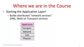
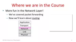
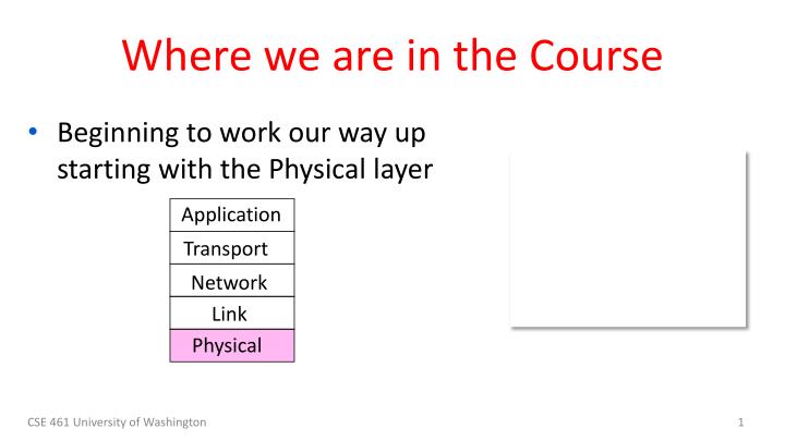
Where we are in the Course. Beginning to work our way up starting with the Physical layer. Application. Transport. Network. Link. Physical. Scope of the Physical Layer. Concerns how signals are used to transfer message bits over a link Wires etc. carry analog signals

E N D
Where we are in the Course • Beginning to work our way up starting with the Physical layer Application Transport Network Link Physical CSE 461 University of Washington
Scope of the Physical Layer • Concerns how signals are used to transfer message bits over a link • Wires etc. carry analog signals • We want to send digital bits 10110… …10110 Signal CSE 461 University of Washington
Topics • Properties of media • Wires, fiber optics, wireless • Simple signal propagation • Bandwidth, attenuation, noise • Modulation schemes • Representing bits, noise • Fundamental limits • Nyquist, Shannon CSE 461 University of Washington
Simple Link Model • We’ll end with an abstraction of a physical channel • Rate (or bandwidth, capacity, speed) in bits/second • Delay in seconds, related to length • Other important properties: • Whether the channel is broadcast, and its error rate Message Delay D, Rate R CSE 461 University of Washington
Message Latency • Latency is the delay to send a message over a link • Transmission delay: time to put M-bit message “on the wire” • Propagation delay: time for bits to propagate across the wire • Combining the two terms we have: CSE 461 University of Washington
Message Latency (2) • Latency is the delay to send a message over a link • Transmission delay: time to put M-bit message “on the wire” T-delay = M (bits) / Rate (bits/sec) = M/R seconds • Propagation delay: time for bits to propagate across the wire P-delay = Length / speed of signals = Length / ⅔c = D seconds • Combining the two terms we have: L = M/R + D CSE 461 University of Washington
Metric Units • The main prefixes we use: • Use powers of 10 for rates, 2 for storage • 1 Mbps = 1,000,000 bps, 1 KB = 210bytes • “B” is for bytes, “b” is for bits CSE 461 University of Washington
Latency Examples • “Dialup” with a telephone modem: • D = 5 ms, R = 56 kbps, M = 1250 bytes • Broadband cross-country link: • D = 50 ms, R = 10 Mbps, M = 1250 bytes CSE 461 University of Washington
Latency Examples (2) • “Dialup” with a telephone modem: D = 5 ms, R = 56 kbps, M = 1250 bytes L = 5 ms+ (1250x8)/(56 x 103) sec = 184 ms! • Broadband cross-country link: D = 50 ms, R = 10 Mbps, M = 1250 bytes L = 50 ms+ (1250x8) / (10 x 106) sec = 51 ms • A long link or a slow rate means high latency • Often, one delay component dominates CSE 461 University of Washington
Bandwidth-Delay Product • Messages take space on the wire! • The amount of data in flight is the bandwidth-delay (BD) product BD = R x D • Measure in bits, or in messages • Small for LANs, big for “long fat” pipes CSE 461 University of Washington
Bandwidth-Delay Example • Fiber at home, cross-country R=40 Mbps, D=50 ms 110101000010111010101001011 CSE 461 University of Washington
Bandwidth-Delay Example (2) • Fiber at home, cross-country R=40 Mbps, D=50 ms BD = 40 x 106x 50 x 10-3 bits = 2000 Kbit = 250 KB • That’s quite a lot of data “in the network”! 110101000010111010101001011 CSE 461 University of Washington
Frequency Representation • A signal over time can be represented by its frequency components (called Fourier analysis) amplitude = Signal over time weights of harmonic frequencies CSE 461 University of Washington
Effect of Less Bandwidth • Fewer frequencies (=less bandwidth) degrades signal Lost! Bandwidth Lost! CSE 461 University of Washington Lost! 14
Signals over a Wire • What happens to a signal as it passes over a wire? • The signal is delayed (propagates at ⅔c) • The signal is attenuated (goes for m to km) • Frequencies above a cutoff are highly attenuated • Noise is added to the signal (later, causes errors) EE: Bandwidth = width of frequency band, measured in Hz CS: Bandwidth = information carrying capacity, in bits/sec CSE 461 University of Washington
Signals over a Wire (2) • Example: 2: Attenuation: Sent signal 3: Bandwidth: 4: Noise: CSE 461 University of Washington
Signals over Fiber Attenuation (dB/km • Light propagates with very low loss in three very wide frequency bands • Use a carrier to send information By SVG: Sassospicco Raster: Alexwind, CC-BY-SA-3.0, via Wikimedia Commons Wavelength (μm) CSE 461 University of Washington
Signals over Wireless • Signals transmitted on a carrier frequency, like fiber (more later) CSE 461 University of Washington
Signals over Wireless (2) • Travel at speed of light, spread out and attenuate faster than 1/dist2 Signal strength A B Distance CSE 461 University of Washington
Signals over Wireless (3) • Multiple signals on the same frequency interfere at a receiver Signal strength A B C Distance CSE 461 University of Washington
Signals over Wireless (4) • Interference leads to notion of spatial reuse(of same freq.) Signal strength A B C Distance CSE 461 University of Washington
Signals over Wireless (5) • Various other effects too! • Wireless propagation is complex, depends on environment • Some key effects are highly frequency dependent, • E.g., multipath at microwave frequencies CSE 461 University of Washington
Wireless Multipath • Signals bounce off objects and take multiple paths • Some frequencies attenuated at receiver, varies with location • Messes up signal; handled with sophisticated methods (§2.5.3) CSE 461 University of Washington
Wireless • Sender radiates signal over a region • In many directions, unlike a wire, to potentially many receivers • Nearby signals (same freq.) interfere at a receiver; need to coordinate use CSE 461 University of Washington
WiFi WiFi CSE 461 University of Washington
Wireless (2) • Microwave, e.g., 3G, and unlicensed (ISM) frequencies, e.g., WiFi, are widely used for computer networking 802.11 b/g/n 802.11a/g/n CSE 461 University of Washington
Topic • We’ve talked about signals representing bits. How, exactly? • This is the topic of modulation Signal 10110… …10110 CSE 461 University of Washington
A Simple Modulation • Let a high voltage (+V) represent a 1, and low voltage (-V) represent a 0 • This is called NRZ (Non-Return to Zero) +V Bits 0 0 1 0 1 1 1 1 0 1 0 0 0 0 1 0 -V NRZ CSE 461 University of Washington
A Simple Modulation (2) • Let a high voltage (+V) represent a 1, and low voltage (-V) represent a 0 • This is called NRZ (Non-Return to Zero) +V Bits 0 0 1 0 1 1 1 1 0 1 0 0 0 0 1 0 -V NRZ CSE 461 University of Washington
Many Other Schemes • Can use more signal levels, e.g., 4 levels is 2 bits per symbol • Practical schemes are driven by engineering considerations • E.g., clock recovery » CSE 461 University of Washington
Clock Recovery • Um, how many zeros was that? • Receiver needs frequent signal transitions to decode bits • Several possible designs • E.g., Manchester coding and scrambling (§2.5.1) 1 0 0 0 0 0 0 0 0 0 … 0 CSE 461 University of Washington
Clock Recovery – 4B/5B • Map every 4 data bits into 5 code bits without long runs of zeros • 0000 11110, 0001 01001, 1110 11100, … 1111 11101 • Has at most 3 zeros in a row • Also invert signal level on a 1 to break up long runs of 1s (called NRZI, §2.5.1) CSE 461 University of Washington
Clock Recovery – 4B/5B (2) • 4B/5B code for reference: • 000011110, 000101001, 111011100, … 111111101 • Message bits: 1 1 1 1 0 0 0 0 0 0 0 1 Coded Bits: Signal: CSE 461 University of Washington
Clock Recovery – 4B/5B (3) • 4B/5B code for reference: • 000011110, 000101001, 111011100, … 111111101 • Message bits: 1 1 1 1 0 0 0 0 0 0 0 1 1 1 1 0 1 1 1 1 1 0 0 1 0 0 1 Coded Bits: Signal: CSE 461 University of Washington
Passband Modulation • What we have seen so far is baseband modulation for wires • Signal is sent directly on a wire • These signals do not propagate well on fiber / wireless • Need to send at higher frequencies • Passband modulation carries a signal by modulating a carrier CSE 461 University of Washington
Passband Modulation (2) • Carrier is simply a signal oscillating at a desired frequency: • We can modulate it by changing: • Amplitude, frequency, or phase CSE 461 University of Washington
Passband Modulation (3) NRZ signal of bits Amplitude shift keying CSE 461 University of Washington Frequency shift keying Phase shift keying
Topic • How rapidly can we send information over a link? • Nyquist limit (~1924) » • Shannon capacity (1948) » • Practical systems are devised to approach these limits CSE 461 University of Washington
Key Channel Properties • The bandwidth (B), signal strength (S), and noise strength (N) • B limits the rate of transitions • S and N limit how many signal levels we can distinguish Bandwidth B Signal S, Noise N CSE 461 University of Washington
Nyquist Limit • The maximum symbol rate is 2B • Thus if there are V signal levels, ignoring noise, the maximum bit rate is: 1 0 1 0 1 0 1 0 1 0 1 0 1 0 1 0 1 0 1 R = 2B log2V bits/sec CSE 461 University of Washington
Claude Shannon (1916-2001) • Father of information theory • “A Mathematical Theory of Communication”, 1948 • Fundamental contributions to digital computers, security, and communications Electromechanical mouse that “solves” mazes! Credit: Courtesy MIT Museum CSE 461 University of Washington
Shannon Capacity • How many levels we can distinguish depends on S/N • Or SNR, the Signal-to-Noise Ratio • Note noise is random, hence some errors • SNR given on a log-scale in deciBels: • SNRdB = 10log10(S/N) S+N 0 N 1 2 3 CSE 461 University of Washington
Shannon Capacity (2) • Shannon limit is for capacity (C), the maximum information carrying rate of the channel: C = B log2(1 + S/N) bits/sec CSE 461 University of Washington
Wired/Wireless Perspective • Wires, and Fiber • Engineer link to have requisite SNR and B • Can fix data rate • Wireless • Given B, but SNR varies greatly, e.g., up to 60 dB! • Can’t design for worst case, must adapt data rate CSE 461 University of Washington
Wired/Wireless Perspective (2) • Wires, and Fiber • Engineer link to have requisite SNR and B • Can fix data rate • Wireless • Given B, but SNR varies greatly, e.g., up to 60 dB! • Can’t design for worst case, must adapt data rate Engineer SNR for data rate Adapt data rate to SNR CSE 461 University of Washington
Putting it all together – DSL • DSL (Digital Subscriber Line, see §2.6.3) is widely used for broadband; many variants offer 10s of Mbps • Reuses twisted pair telephone line to the home; it has up to ~2 MHz of bandwidth but uses only the lowest ~4 kHz CSE 461 University of Washington
DSL (2) • DSL uses passband modulation (called OFDM §2.5.1) • Separate bands for upstream and downstream (larger) • Modulation varies both amplitude and phase (called QAM) • High SNR, up to 15 bits/symbol, low SNR only 1 bit/symbol 0-4 kHz 26 – 138 kHz 143 kHz to 1.1 MHz Up to 12 Mbps Voice Up to 1 Mbps ADSL2: Freq. Upstream Telephone Downstream CSE 461 University of Washington