Download
1 / 58
580 likes | 589 Views
Spatial Current Structure Observed with a Validated HF Radar System: The Influence of Local Forcing, Stratification, and Topography on the Inner Shelf. Josh Kohut Scott Glenn Hugh Roarty Bob Chant Dale Haidvogel Rutgers University Jeff Paduan Naval Postgraduate School.

E N D
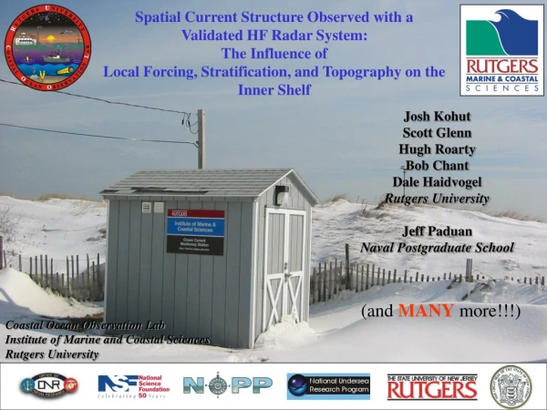
Spatial Current Structure Observed with a Validated HF Radar System: The Influence of Local Forcing, Stratification, and Topography on the Inner Shelf Josh Kohut Scott Glenn Hugh Roarty Bob Chant Dale Haidvogel Rutgers University Jeff Paduan Naval Postgraduate School (and MANY more!!!) Coastal Ocean Observation Lab Institute of Marine and Coastal Sciences Rutgers University
ROW 2 Meeting • Role of antenna pattern distortion on system accuracy • Kohut, J.T. and S.M. Glenn. 2003. Improving HF radar surface current • measurements with measured antenna beam patterns. - accepted Journal of • Atmospheric and Oceanic Technology. • The Long-Range 5 MHz network setup • Roarty, H. J., J. T. Kohut, and S. M. Glenn. 2003. Intercomparison of an • ADCP, ADP, standard and long-range HF radar: Influence of horizontal and • vertical shear. IEEE Current Measurement Proceedings. • Introduced seasonal and event scale variability over the • inner shelf (25 MHz System) • mean fields and transient fields
1998 1999 2000 2001 2002 Test
Seasonal Variability: Data Annual Mean
Seasonal Variability: Data 30 25 20 15 10 5 0 Temperature (ºC) Winds HF radar ADCP Stratified Mixed 150 200 250 300 350 35 85 Time (year-day)
Seasonal Variability Stratified Regime Response
Seasonal Variability: Stratified Regime Wind Forcing Number of Hourly Occurrences Wind Speed (m/s) Wind Direction (degrees CW from true north)
Seasonal Variability: Stratified Regime Stratified Water Column Complex Correlation 1.0 0.9 0.8 0.7 0.6 0.5 0.4 0.3 0.2 0.1 0.0 0 3 4 5 6 7 8 9 10 Depth (m) 1.0
Seasonal Variability: Stratified Regime Upwelling Response Mean (U) Spatial Structure • Strong mean flow
Bathymetric Variability on Upwelling Seasonal Variability: Stratified Regime 1 m/s current velocity Along shore subsurface deltas cause upwelling to be 3d, not 2d. wind
Seasonal Variability: Stratified Regime Downwelling Response Mean (U) Spatial Structure • Strong mean flow
Seasonal Variability: Stratified Regime Downwelling Regime Sea-Surface Temperature Correlation 0.0 0.1 0.2 0.3 0.4 0.5 0.6 0.7 0.8 0.9 1.0 Correlation
Seasonal Variability: Stratified Regime
Seasonal Variability Mixed Regime Forcing
Seasonal Variability: Mixed Regime Wind Forcing Wind Speed (m/s) Number of Hourly Occurrences Wind Direction (degrees CW from true north)
Seasonal Variability: Mixed Regime Mixed Water Column Complex Correlation 1.0 0.9 0.8 0.7 0.6 0.5 0.4 0.3 0.2 0.1 0.0 0 3 4 5 6 7 8 9 10 Depth (m) 1.0
Seasonal Variability: Mixed Regime = k u z K * k u = * l f ( ) - k u u = 2 1 u * æ ö z ç ÷ ln 2 ç ÷ z è ø 1 Frictional Layer 300 250 200 150 100 50 0 Linear eddy viscosity Frictional Velocity Depth Scale (m) Frictional Length Scale 240 260 280 300 320 340 360 Time (year-day)
Seasonal Variability Mixed Regime Bottom topography
Seasonal Variability: Mixed Regime Principle Components dh dL 5 10 15 20 25 30 35 Topography 20 km 5 km minimize : Depth (m) h = depth L = horizontal scale
Seasonal Variability: Mixed Regime 3.0 2.5 2.0 1.5 1.0 0.5 0.0 Depth Gradient (m/km) Influence of Gradient Maximum 30 20 10 0 -10 -20 -30 -40 -50 -60 Angular Offset (degrees) Negative angle : Principle axis right of topography
Storm Response
Storm Event Forcing Floyd’s Track
Storm Event Forcing Wind (m/s) Wind speed (m/s) Inertail amp (m/s) Pressure (mbars) Rainfall (cm/hour) Time (year-day)
Storm Event Response Wind Surface 3m 10m
Storm Event Response Surface 3m 4m 5m 6m 7m 8m 9m 10m Depth-Averaged CW CCW Time (year-day)
Storm Event Response Near-Inertial Response Angle 4 3 2 1 0 -1 -2 -3 -4 Depth (m) Phase (degrees) 25 cm/s Amplitude (cm/s)
Storm Event Models ¶ ¶ h t t u = - + + - wx bx g fv ¶ r r t dx H H Single Layer Model Equations t t ¶ ¶ h v wy by = - - + - g fu ¶ r r t dy H H Pressure Gradient Bottom Stress Depth-averaged Acceleration Wind Stress Coriolis w TOGA-COARE2.6 algorithm (Fairall et al., 1996) Local Wind (10m) Air temperature Sea temperature relative humidity t = r 2 u b * ADCP/HF Radar ADCPWindsInferred
Along-shore Velocity (cm/s) Acceleration Pressure GradientCoriolis Bottom stress Wind Stress Along-shore Momentum Balance
Storm Response Larger Spatial Scales
NEOS Northeaster Oct 16, 2002 GoMOOS NJSOS MVCO LEO 15
Spatial Maps 10/16/2002 0700 GMT RUC Wind and Pressure Analysis CODAR Surface Currents 1002 mb Contour resolution – 1 mb
RUC Wind and Pressure Analysis CODAR Surface Currents L L 10/16/2002 1500 GMT 991 mb Contour resolution – 1 mb
RUC Wind and Pressure Analysis CODAR Surface Currents L L 10/16/2002 1800 GMT 989 mb Contour resolution – 1 mb
RUC Wind and Pressure Analysis CODAR Surface Currents L L 10/17/2002 0000 GMT 992 mb Contour resolution – 1 mb
NEOS: Existing Sub-Regional Observatories
NVODS & OPeNDAP CODAR Pilot Project (Peter Cornillon and Dave Ullman) Develop Capability to Provide CODAR Data from Multiple Systems in a Seamless Manner. • Client requests data from a user selected region that may contain more than one CODAR system. • Aggregation server: Combines data from a number of different CODAR systems and provides to client. • http://www.nvods.org; http://www.opendap.org
Current operational prediction CODE drifter CODAR based prediction