SYSTEM IDENTIFICATION
v ( t ). disturbance (not observed). System. y ( t ). u ( t ). output (observed). input (observed). { v ( k )}. System. { y ( k )}. { u ( k )}. SYSTEM IDENTIFICATION. The System Identification Problem is to estimate a model of a system based on input-output data. Basic Configuration.

SYSTEM IDENTIFICATION
E N D
Presentation Transcript
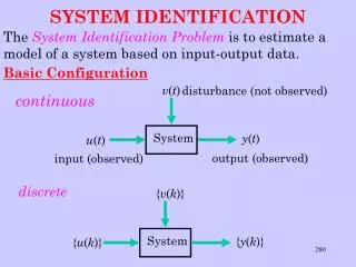
v(t) disturbance (not observed) System y(t) u(t) output (observed) input (observed) {v(k)} System {y(k)} {u(k)} SYSTEM IDENTIFICATION The System Identification Problemis to estimate a model of a system based on input-output data. Basic Configuration continuous discrete
If we assume the system is linear we can write:- using standard z-transform notation We observe an input number sequence(a sampled signal) {u(k)} = {u(0), u(1), ..., u(k), ..., u(N)} and an output sequence {y(k)} = {y(0), y(1), ..., y(k), ..., y(N)}
V(z) + Y(z) G(z) U(z) (z) H(z) white noise V(z) filter disturbance + Y(z) G(z) U(z) output input process The disturbance v(k) is often considered as generated by filtered white noise :- giving the description:
(z) V(z) H(z) Y(z) U(z) + G(z) Parametric Models ARX model (autoregressive with exogenous variables) where
estimate (parameters) and represents an extra delay of n sampling instants. giving the difference equation: identification problem determinen, na, nb (structure)
ARMAX model (autoregressive moving average with exogenous variables) (z) V(z) H(z) Y(z) U(z) + G(z) where
estimate (parameters) giving the difference equation: identification problem determine n, na, nb, nc (structure)
y(t) u(t) Process - e(t,) + Predictor with adjustable parameters Algorithm for minimising some function of e(t,) General Prediction Error Approach Predictor based on a parametric model Algorithmoften based on a least squares method.
Consistency A desirable property of an estimate is that it converges to the true parameter value as the number of observations N increases towards infinity. This property is called consistency Consistency is exhibited by ARMAX model identification methods but not by ARX approaches (the parameter values exhibit bias).
Example of MATLAB Identification Toolbox Session Input and Output Data of Dryer Model
MATLAB statements and results: (ARX n, na = 2, nb = 2)
PERFORMANCE ASSESSMENT & UPDATING MECHANISM K J Astrom disturbances regulator parameters fast varying REGULATOR PROCESS ref + _ parameters slowly varying outputs (fast varying) ADAPTIVE CONTROL
Adaptive controlis a special type of nonlinear control in which the states of the process can be separated into two categories:- (i) slowly varying states(viewed as parameters (ii) fast varying states(compensated by standard feedback) In adaptive control it is assumed that there is feedback from the system performance which adjusts the regulator parameters to compensate for the slowly varying process parameters.
An adaptive controller will contain :- Adaptive Control Problem • characterization of desired closed-loop performance (reference model or design specifications) • control law with adjustable parameters • design procedure • parameters updating based on measurements • implementation of the control law (discrete or continuous)
operating conditions gain schedule regulator parameters command signal y u regulator process control signal output Overview of Some Adaptive Control Schemes Gain Scheduling The regulator parameters are adjusted to suit different operating conditions. Gain scheduling is an open-loop compensation.
parameters K, Ti, Td + PID controller Process _ Auto-tuning PID controllers are traditionally tuned using simple experiments and empirical rules. Automatic methods can be applied to tune these controllers. (i) experimental phaseusing test signals; then:- (ii) use of standard rulesto compute PID parameters.
model ideal output ym regulator parameters adjustment mechanism uc y u regulator process actual output MRAS Model Reference Adaptive Systems
The parameters of the regulator are adjusted such that the error e = y - ym becomes small. The key problem is to determine an appropriate adjustment mechanism and a suitable control law. MIT rule adjustment mechanism where determines the adaptation rate. This rule changes the parameters in the direction of the negative gradient of e2
Combining the MIT rule with the control law: and computing the sensitivity derivatives produces the scheme: ym model filter integrator _ e + multiplier + process uc u y _ multiplier Note: steady-state will be achieved when the input to the integrator becomes zero. That is when y = ym
process parameters design estimation regulator parameters uc y u regulator process actual output STR Self Tuning Regulators
The process parameters are updated and the regulator parameters are obtained from the solution of a design problem. The adaptive regulator consists of two loops:- • (i)inner loopconsisting of the process and a linear feedback regulator • (ii) outer loopcomposed of a parameter estimator (recursive) and a design calculation. (To obtain good estimates it is usually necessary to introduce perturbation signals) • Two problems:- • (i) underlying design problem • (ii) real time parameter estimation problem
w(t) v(t) y(t) u(t) x(t) SYSTEM INTRODUCTION TO THE KALMAN FILTER State Estimation Problem Vectors w(t) and v(t) are noise terms, representing unmeasured system disturbancesandmeasurement errorsrespectively. They are assumed to be independent, white,Gaussian, and to have zero mean. In mathematical terms:-
where Q and R are symmetric and non negative definite covariance matrices. (E is the expectation operator) Only u(t) and y(t) are assessable. The state estimation problemis to estimate the states x(t) from a knowledge of u(t) and y(t). (and assuming we know A, B, G, C, D, Q, and R).
y(t) u(t) SYSTEM x(t) D A + + B C _ u(t) + y(t) L(t) FILTER Filter equation :- Construction of the Kalman-Bucy Filter
Filter equation :- The estimation problem is now to find L(t) such that the error between the real states x(t) and the estimated states is minimized. This can be formulated as: R E Kalman L(t) is a time dependent matrix gain.
It can be shown that the optimum state estimation problem: subject to: is the dual of the optimum regulator problem: subject to: Duality Between the Optimum State Estimation Problem and the Optimum Regulator Problem
Thus L(t) can be obtained by solving the matrix Ricatti equation: Furthermore for large measurement times L(t) converges to: a constant matrix gain.
Example: produces:
giving the filter equations: where l1 = 0.5562, l2 = 0.1547
w(t) v(t) y(t) x1 x2 u(t) = 0 + + -1 SYSTEM -1 _ + + + l1 l2 FILTER