Download
1 / 16
160 likes | 256 Views
Explore insights from the 2006 Bologna meeting on detecting Warm-Hot Intergalactic Medium (WHIM) in Gamma-Ray Burst (GRB) spectra. Discussions revolve around energy, distances, line distributions, and simulations, offering a comprehensive overview of the WHIM detection process in GRB data. Discover valuable findings and methodologies presented by experts in the field to enhance understanding and detection capabilities in analyzing GRB spectra for WHIM absorption features.

E N D
ESTREMO/WFXRT: Meeting on scientific requirements – Bologna, 2006 May 4-5 Detecting WHIM in GRB spectra • Corsi, L. Piro & WHIM Working Group
Summary • Why GRBs? • Updated simulations (Viel 2006) - that include OVII k-, OVII k-, OVIII and FeXVII - tested on a typical GRB spectrum; • Number distribution of bright GRBs ESTREMO/WFXRT: Meeting on scientific requirements – Bologna, 2006 May 4-5
GRBs: energy and distances The brightest (Liso=1053-54 erg/s) and most distant sources in the Universe (z = 0.16 - 6.3): sufficiently bright and distant to be good candidates as background sources to detect WHIM absorption features Mean redshift: <z> = 2.8 Prompt fluence: <F15-150 keV> = 2.410-6 erg cm-2 80% of GRBs have X-ray afterglows with fluences around 10%-1000% of the prompt fluence 2.4x10⁻⁷ erg cm-2 < F 0.3-10 keV < 2.4x10⁻⁵ erg cm-2 (O’Brien et al. 2006) (Jackobsson et al. 2005) ESTREMO/WFXRT: Meeting on scientific requirements – Bologna, 2006 May 4-5
Using the typical spectral shape of an X-ray afterglow we can compute, for different values of the afterglow luminosity, the expected counts for 60 ks integration time Estimated using BeppoSAX results, confirmed by Swift Knowing the number of counts from the continuum (X-ray afterglow) we can compute the minimum EW to have a detection at the 5 level, having an energy resolution E= 2 eV: S/N = EW (Counts/eV @ 0.5keV / E)0.5 5 WHIM absorption features: line @0.5 keV on a background GRB afterglow ESTREMO/WFXRT: Meeting on scientific requirements – Bologna, 2006 May 4-5
WHIM absorption features from the hydro simulation We have considered 5 line of sights generated from the output of the new hydrodynamical simulation (Viel 2006) and computed the EW, the mean Energy and the . An example: LOS 1 OVII k- OVII k- OVIII FeXVII ESTREMO/WFXRT: Meeting on scientific requirements – Bologna, 2006 May 4-5
ESTREMO/WFXRT: Meeting on scientific requirements – Bologna, 2006 May 4-5
Distribution • 1 filament with EW 0.1eV (= 50 km/s) in OVII k- up to z=0.5 (i.e. 2 per unit z): in agreement with what expected from Viel et al. (2003). From Hellsten et al.: about 10 per unit z; • 1 filament with EW 1/3 x 0.1eV (= 17 km/s) in OVIII up to z=0.5 (i.e. 2 per unit z). From Viel et al. 2003: 0.6 per unit redshift. From Hellsten et al.: about 10 per unit z; • The same filament gives OVIII line with a mean EW of about 1/3 of the OVII k-α one and FeXVII line with EW of about ½ the OVII k-α. ESTREMO/WFXRT: Meeting on scientific requirements – Bologna, 2006 May 4-5
Detecting WHIM in GRB spectra • A routine to include the model in XSPEC has been developed. It is now available on the web page (tested for XSPEC11). Multiplicative model. The user can select the LOS and the ION. Applying more times the model one can simulate the whole spectrum; • Convolved with 2 eV resolution matrix; • The background source spectrum is a typical GRB one: absorbed power-law with photon index 2, NH=2e20 cgs, fluence of 4e-6 cgs between 60 s and 60 ks. ESTREMO/WFXRT: Meeting on scientific requirements – Bologna, 2006 May 4-5
OVII k- z=0.062 EW=0.33 eV OVII k- z=0.46 eV EW= 0.11 eV Fe XVII z=0.062 EW=0.21 eV OVII k- z=0.062 EW=0.18 eV
OVII k- z=0.46 EW=0.093 eV OVII k- z=0.26 EW=0.095 eV OVII k- z=0.36 EW=0.089 eV
Fe XVII z=0.35 EW=0.35 eV OVII k- z=0.061 EW=0.19 eV - 10 - 20
OVII k- z=0.16 EW=0.12 eV OVII k- z=0.1 EW=0.19 eV
How many afterglows? We are interested in the logN-logS of GRB X-ray afterglows (S=fluence): • Method 1: derive it directly from afterglow observations, assuming that the sample is unbiased so that one can normalize the observed distribution to 1000 GRB/yr (expected GRB rate in all the sky); • Method 2: adopt an afterglow-to-prompt ratio and use the logN-logS of the prompt: 2a - use the prompt X (better than gamma-rays because stronger correlation with X-ray afterglow); 2b - use the prompt gamma (logN-logS better sampled vs prompt X) ESTREMO/WFXRT: Meeting on scientific requirements – Bologna, 2006 May 4-5
X-ray afterglow fluence distribution: comparing methods 1-2a/b F. Fiore, first Rome meeting 1000 GRB yr-1 Using the mean value for the ratio prompt X-ray fluence / X-ray afterglow flux @ 11 hrs and the WFC logN-logS, we can compute the number of bursts per yr observable with a FOV of 3sr 100 sec ESTREMO/WFXRT: Meeting on scientific requirements – Bologna, 2006 May 4-5
Conclusions • In ¼ of the sky: • we expect to see about 10 GRBs per year having an X-ray afterglow fluence of the order of 4e-6 cgs typical case: detection of OVII k- lines; best case: detection of OVII k- lines plus FeXVII or OVII k-; • we expect to see about 3 GRBs per year having an X-ray afterglow fluence of the order of 1e-5 cgs typical case: detection of 2 IONs, OVII k- & OVII k- / FeXVII / OVIII; best case: detection of all of the 4. ESTREMO/WFXRT: Meeting on scientific requirements – Bologna, 2006 May 4-5