Download

1 / 37
370 likes | 485 Views
Informed Search. Modified by M. Perkowski. Yun Peng. h. a. g. b. c. d. e. i. h= 1. h=2. h=1. h=1. h=0. h=1. h=1. f. h=0. Informed Methods Add Domain-Specific Information.

E N D
InformedSearch Modified by M. Perkowski. Yun Peng
h a g b c d e i h=1 h=2 h=1 h=1 h=0 h=1 h=1 f h=0 Informed Methods Add Domain-Specific Information • Informed Methods add domain-specific information to select what is the best path to continue searching along • They define a heuristic function, h(n), that estimates the "goodness" of a node n with respect to reaching a goal. • Specifically, h(n) = estimated cost (or distance) of minimal cost path from n to a goal state. • h(n) is about cost of the future search, g(n) past search • h(n) is an estimate (rule of thumb), based on domain-specific information that is computable from the current state description. • Heuristics do not guarantee feasible solutions and are often without theoretical basis.
Heuristics • Examples: • Missionaries and Cannibals: Number of people on starting river bank • 8-puzzle: Number of tiles out of place (i.e., not in their goal positions) • 8-puzzle: Sum of Manhattan distances each tile is from its goal position • 8-queen: # of un-attacked positions – un-positioned queens • In general: • h(n) >= 0 for all nodes n • h(n) = 0 implies that n is a goal node • h(n) = infinity implies that n is a deadend from which a goal cannot be reached
Best First Search • Best First Search orders nodes on the OPEN list by increasing value of an evaluation function, f(n) , that incorporates domain-specific information in some way. • Example of f(n): • f(n) = g(n) (uniform-cost) • f(n) = h(n) (greedy algorithm) • f(n) = g(n) + h(n) (algorithm A) • This is a generic way of referring to the class of informed methods. Thus, uniform-cost, breadth-first, greedy and A are special cases of Best First Search
i h a g b c d e h=4 h=2 h=1 h=1 h=0 h=1 h=1 f h=0 Greedy Search • Evaluation function f(n) = h(n), sorting open nodes by increasing values of f. • Selects node to expand believed to be closest (hence it's "greedy") to a goal node (i.e., smallest f = h value) • Not admissible, as in the example. Assuming all arc costs are 1, then Greedy search will find goal f, which has a solution cost of 5, while the optimal solution is the path to goal i with cost 3. • Not complete (if no duplicate check) Minimal solution of cost 3 Solution found of cost 5
Beam search • Idea = to limit the size of OPEN list. • Use an evaluation function f(n) = h(n), but the maximum size of the list of nodes is k, a fixed constant • Only keeps k best nodes as candidates for expansion, and throws the rest away • More space efficient than greedy search, but may throw away a node that is on a solution path • Not complete • Not admissible
D Algorithm A 8 S 8 5 1 • Algorithm A uses as an evaluation function f(n) = g(n) + h(n) • The h(n) term represents a “depth-first“ factor in f(n) • g(n) = minimal cost path from the start state to state n generated so far • The g(n) term adds a "breadth-first" component to f(n). • Ranks nodes on OPEN list by estimated cost of solution from start node through the given node to goal. • Completeness and admissibility depends on h(n) 1 5 A B C 8 9 3 5 1 4 G 9 f(D)=4+9=13 f(B)=5+5=10 f(C)=8+1=9 C is chosen next to expand as having the smallest value of f Observe that there is no constraint on h g(n) h(n)
Algorithm A OPEN := {S}; CLOSED := {}; repeat Select node n from OPEN with minimal f(n) and place n on CLOSED; if n is a goal node exit with success; Expand(n); For each child n' of n do compute h(n'), g(n')=g(n)+ c(n,n'), f(n')=g(n')+h(n'); if n' is not already on OPEN or CLOSED then put n’ on OPEN; set backpointer from n' to n elseif n' is already on OPEN or CLOSED and if g(n') is lower for the new version of n' then discard the old version of n‘; Put n' on OPEN; set backpointer from n' to n until OPEN = {}; exit with failure
Algorithm A* • Algorithm A with constraint that h(n) <= h*(n) • This is called the admissible heuristic. • h*(n) = true cost of the minimal cost path from n to any goal. • g*(n) = true cost of the minimal cost path from S to n. • f*(n) = h*(n)+g*(n) = true cost of the minimal cost solution path from S to any goal going through n. • h is admissible when h(n) <= h*(n) holds. • Using an admissible heuristic guarantees that the first solution found will be an optimal one. • A* is completewhen: • (1) the branching factor is finite, and • (2) every operator has a fixed positive cost : • i.e. the total # of nodes with f(.) <= f*(goal) is finite • A* is admissible Observe that we can calculate h* when the whole tree is already known. Expanding the whole tree can be then used to define better function h.
Some Observations on A* • Null heuristic: If h(n) = 0 for all n, then this is an admissible heuristic and A* acts like Uniform-Cost Search. • Thus Uniform-Cost is a special case of A* • Better heuristic: If h1(n) <= h2(n) <= h*(n) for all non-goal nodes, then h2is a better heuristic than h1 • If A1* uses h1, and A2* uses h2, then every node expanded by A2* is also expanded by A1*. • In other words, A1 expands at least as many nodes as A2*. • We say that A2* is better informed than A1*. • The closer h is to h*, the fewer extra nodes that will be expanded • Perfect heuristic: • If h(n) = h*(n) for all n, then only the nodes on the optimal solution path will be expanded. • So, no extra work will be performed.
start state parent pointer 8 0 S arc cost 8 1 5 1 A B 4 C 5 8 3 8 3 9 h value 7 4 3 g value D E 4 8 G 9 0 goal state Example search space: please note values of g and h in nodes f(n) = g(n) + h(n) Optimal path with cost 9
start state parent pointer 8 0 S arc cost 8 1 5 1 A B 4 C 5 8 3 8 3 9 h value 7 4 5 g value D E 4 8 G 9 0 goal state f*(n) 9 10 9 13 inf inf 0 Example search space h*(n)=9 Accurate prediction n g(n) h(n) f(n) h*(n) S 0 8 8 9 A 1 8 9 9 B 5 4 9 4 C 8 3 11 5 D 4 inf inf inf E 8 inf inf inf G 9 0 9 0 h*(n)=9 h*(n)=4 h*(n)=5 h*(n)=0 h*(n)=inf h*(n)=inf f(n) = g(n) + h(n)
Using f*(n) we would be able to find directly the optimum solution. f(n) = g(n) + h(n) Example f*(n) 9 10 9 13 inf inf 0 n g(n) h(n) f(n) h*(n) S 0 8 8 9 A 1 8 9 9 B 5 4 9 4 C 8 3 11 5 D 4 inf inf inf E 8 inf inf inf G 9 0 9 0 • h*(n) is the (hypothetical) perfect heuristic. • Since h(n) <= h*(n) for all n, h is admissible • Optimal path = S B G with cost 9. • Optimal path would be found directly if we would be able to calculate h*
start state parent pointer 8 0 S arc cost 8 1 5 A B 4 C 3 1 8 5 8 3 9 h value 7 4 5 g value D E G 0 4 8 9 goal state Greedy Algorithm f(n) = h(n) node exp. OPEN list {S(8)} S {C(3) B(4) A(8)} C {G(0) B(4) A(8)} G {B(4) A(8)} • Solution path found is S C G with cost 13. • 3 nodes expanded. • Fast, but not optimal.
start state parent pointer 8 0 S arc cost 8 1 5 1 A B 4 C 5 8 3 8 3 9 h value 7 4 5 g value D E 4 8 G 9 0 goal state A* Search f(n) = g(n) + h(n) node exp. OPEN list {S(8)} S {A(9) B(9) C(11)} A {B(9) G(10) C(11) D(inf) E(inf)} B {G(9) G(10) C(11) D(inf) E(inf)} G {C(11) D(inf) E(inf)} • Solution path found is S B G with cost 9 • 4 nodes expanded. • Still pretty fast. And optimal, too.
Proof of the Optimality of A* • Let l* be the optimal solution path (from S to G), let f* be its cost • At any time during the search, one or more node on l* are in OPEN • We assume that A* has selected G2, a goal state with a suboptimal solution (g(G2) > f*). • We show that this is impossible. • Let node n be the shallowest OPEN node on l* • Because all ancestors of n along l* are expanded, g(n)=g*(n) • Because h(n) is admissible, h*(n)>=h(n). Then f* =g*(n)+h*(n) >= g*(n)+h(n) = g(n)+h(n)= f(n). • If we choose G2 instead of n for expansion, f(n)>=f(G2). • This implies f*>=f(G2). • G2 is a goal state: h(G2) = 0, f(G2) = g(G2). • Therefore f* >= g(G2) • Contradiction. Read it at home. See Luger book
Iterative Deepening A* (IDA*) • Idea: • Similar to IDDF: • In IDDF search at each iteration is bound by the depth, • In IDA* search is bound by the current f_limit • At each iteration, all nodes with f(n) <= f_limit will be expanded (in DF fashion). • If no solution is found at the end of an iteration, increase f_limit and start the next iteration • f_limit: • Initialization: f_limit := h(s) • Increment: at the end of each (unsuccessful) iteration, f_limit := max{f(n)|n is a cut-off node} • Goal testing: • test all cut-off nodes until a solution is found • select the least cost solution if there are multiple solutions • IDA* is Amissible if h is admissible
What’s a good heuristic? • As we remember if h1(n) < h2(n) <= h*(n) for all n, then h2 is better than h1 • We say, h2 dominates h1. • Relaxing the problem: • remove constraints to create a (much) easier problem; • use the solution cost for this easier problem as the heuristic function h • Combining heuristics: • take the max of several admissible heuristics to create h: • still have an admissible heuristic, and it’s better! • Use statistical estimates to compute h: may lose admissibility • Identify good features, then use a learning algorithm to find a heuristic function: • also may lose admissibility
Automatic generation of h functions • Original problem PRelaxed problem P' A set of constraints removing one or more constraints P is complexP' becomes simpler • Use cost of a best solution path from n in P' as h(n) for P • Admissibility: h* h cost of best solution in P>=cost of best solution in P' Solution space of P Solution space of P'
Automatic generation of h functions • Example:8-puzzle • Constraints: to move a tile from cell A to cell B there are 3 conditions as follows: cond1: there is a tile on A cond2: cell B is empty cond3: A and B are adjacent (horizontally or vertically) • Removing cond2 we obtain function h2: h2 (sum of Manhattan distances of all misplaced tiles) • Removing cond2 and cond3 we obtain function h1: h1 (# of misplaced tiles) • Removing cond3 we obtain function h3: h3, a new heuristic function calculated as below h1(start) = 7 h2(start) = 18 h3(start) = 7
Relaxing the problem: • remove constraints to create a (much) easier problem; • use the solution cost for this easier problem as the heuristic function h h3: repeat if the current empty cell A is to be occupied by tile x in the goal, move x to A. Otherwise, move into A any arbitrary misplaced tile. until the goal is reached • It can be checked that: h2>= h3 >= h1 h1(start) = 7 h2(start) = 18 h3(start) = 7 • Use cost of a best solution path from n in P' as h(n) for P
Another Example: Traveling Salesman Problem. • A legal tour is a (Hamiltonian) circuit • Variant 1: It is a connectedsecond degree graph (each node has exactly two adjacent edges) • Removing the connectivity constraint leads to h1: • find the cheapest second degree graph from the • given graph • (with o(n^3) complexity) The given complete graph A legal tour Other second degree graphs
The given graph A legal tour • Variant 2: legal tour is a spanning tree (when an edge is removed) with the constraint that each node has at most 2 adjacent edges) Removing the constraint leads to h2: find the cheapest minimum spanning tree from the given graph (with O(n^2/log n) Other spanning trees • Relaxing the problem: • remove constraints to create a (much) easier problem; • use the solution cost for this easier problem as the heuristic function h
Complexity of A* search • In general: • exponential time complexity • exponential space complexity • For subexponential growth of # of nodes expanded, we need |h(n)-h*(n)| <= O(log h*(n)) for all n For most problems we have|h(n)-h*(n)| <= O(h*(n) • Relaxing optimality can be done using one of the following methods: • Method 1. Weighted evaluation function f(n) = (1-w)*g(n)+w*h(n) w=0: uniformed-cost search w=1: greedy algorithm w=1/2: A* algorithm when w > ½, search is more depth-first (radical) than A* Read this slide at home and in book
Method 2. Dynamic weighting f(n)=g(n)+h(n)+ [1- d(n)/N]*h(n) d(n): depth of node n N: anticipated depth of an optimal goal at beginning of search: << N encourages DF search when close to the end: back to A* It is -admissible (solution cost found is <= (1+ ) solution found by A*) Read at home and in book
Read at home and in book Method 3: • : another -admissible algorithm select n from OPEN for expansion if f(n) <= (1 + )*smallest f value among all nodes in OPEN • Select n if it is a goal • Otherwise select randomly or with smallest h value Method 4: • Pruning OPEN list (cutting-off): • Find a solution using some quick but non-admissible method (e.g., greedy algorithm, hill-climbing, neural networks) with cost f+ • Do not put a new node n on OPEN unless f(n) <= f+ • Admissible: suppose f(n) > f+ >= f*, the least cost solution sharing the current path from s to n would have cost g(n) + h*(n) >= g(n) + h(n) = f(n)>f*
Iterative Improvement Search • Another approach to search involves starting with an initial guess at a solution and gradually improving it. • Some examples: • Hill Climbing • Simulated Annealing • Genetic algorithm
Hill Climbing on a Surface of States Height Defined by Evaluation Function n n’
Hill Climbing Search • If there exists a successor n’ for the current state n such that • h(n’) < h(n) • h(n’) <= h(t) for all the successors t of n, then move from n to n’. Otherwise, halt at n. • Looks one step ahead to determine if any successor is better than the current state; • if there is, move to the best successor. • Similar to greedy search in that it uses h only, but does not allow backtracking or jumping to an alternative pathsince it doesn’t “remember” where it has been. • OPEN = {current-node} • Not complete since the search will terminate at "local minima," "plateaus," and "ridges."
start h = 0 goal h = 4 2 5 5 6 1 4 6 4 8 5 4 2 5 5 6 7 3 2 1 6 7 1 8 5 8 3 3 7 6 4 7 1 5 8 7 8 3 3 3 2 7 5 1 6 4 8 1 4 h = 3 h = 1 3 4 2 2 2 h = 2 h = 3 4 Hill climbing example Here or here? Selected this because of look ahead f(n) = (number of tiles out of place)
Drawbacks of Hill-Climbing • Problems: • Local Maxima: • Plateaus: the space has a broad flat plateau with a singularity as it’s maximum • Ridges: steps to the North, East, South and West may go down, but a step to the NW may go up. • Remedy: • Random Restart. • Multiple HC searches from different start states • Some problems spaces are great for Hill Climbing and others horrible.
6 2 7 4 8 6 3 1 2 4 7 3 8 6 5 1 8 6 1 2 5 7 8 3 3 1 2 5 7 4 4 5 3 1 2 5 7 4 8 6 Example of a local maximum -4 start goal -4 0 -3 -4
Simulated Annealing • Simulated Annealing (SA) exploits an analogy between the way in which a metal cools and freezes into a minimum energy crystalline structure (the annealing process) and the search for a minimum in a more general system. • Each state n has an energy value f(n), where f is an evaluation function • SA can avoid becoming trapped at local minimum energy state by introducing randomness into search • so that it not only accepts changes that decreases state energy, but also some that increase it. • SAs use a a control parameter T, which by analogy with the original application is known as the system “temperature” irrespective of the objective function involved. • T starts out high and gradually (very slowly) decreases toward 0.
Algorithm for Simulated Annealing current := a randomly generated state; T := T_0 /* initial temperature T0 >>0 */ forever do if T <= T_end then return current; next := a randomly generated new state; /* next != current */ = f(next) – f(current); current := next with probability ; T := schedule(T); /* reduce T by a cooling schedule */ Commonly used cooling schedule • T := T * alpha where 0 < alpha < 1 is a cooling constant • T_k := T_0 / log (1+k)
Observation with Simulated Annealing • Probability of the system is at any particular state depends on the state’s energy (Boltzmann distribution) • If time taken to cool is infinite then So statistically the best solution is found
population selection of parents for reproduction (based on a fitness function) parents reproduction (cross-over + mutation) next generation of population Genetic Algorithms • Emulating biological evolution (survival of the fittest by natural selection process ) • Population of individuals (each individual is represented as a string of symbols: genes and chromosomes) • Fitness function: estimates the goodness of individuals • Selection: only those with high fitness function values are allowed to reproduce • Reproduction: • crossover allows offspring to inherit good features from their parents • mutation (randomly altering genes) may produce new (hopefully good) features • bad individuals are throw away when the limit of population size is reached • To ensure good results, the population size must be large
Informed Search Summary • Best-first search is general search where the minimum cost nodes (according to some measure) are expanded first. • Greedy search uses minimal estimated cost h(n) to the goal state as measure. This reduces the search time, but the algorithm is neither complete nor optimal. • A* search combines uniform-cost search and greedy search: f(n) = g(n) + h(n) and handles state repetitions and h(n) never overestimates. • A* is complete, optimal and optimally efficient, but its space complexity is still bad. • The time complexity depends on the quality of the heuristic function. • IDA* reduces the memory requirements of A*. • Hill-climbing algorithms keep only a single state in memory, but can get stuck on local optima. • Simulated annealing escapes local optima, and is complete and optimal given a slow enough cooling schedule (in probability). • Genetic algorithms escapes local optima, and is complete and optimal given a long enough evolution time and large population size.