Informed Search
Informed Search. ECE457 Applied Artificial Intelligence Fall 2007 Lecture #3. Outline. Heuristics Informed search techniques More on heuristics Iterative improvement Russell & Norvig, chapter 4 Skip “Genetic algorithms” pages 116-120 (will be covered in Lecture 12).

Informed Search
E N D
Presentation Transcript
Informed Search ECE457 Applied Artificial Intelligence Fall 2007 Lecture #3
Outline • Heuristics • Informed search techniques • More on heuristics • Iterative improvement • Russell & Norvig, chapter 4 • Skip “Genetic algorithms” pages 116-120 (will be covered in Lecture 12) ECE457 Applied Artificial Intelligence R. Khoury (2007) Page 2
Recall: Uninformed Search • Travel blindly until they reach Bucharest ECE457 Applied Artificial Intelligence R. Khoury (2007) Page 3
An Idea… • It would be better if the agent knew whether or not the city it is travelling to gets it closer to Bucharest • Of course, the agent doesn’t know the exact distance or path to Bucharest (it wouldn’t need to search otherwise!) • The agent must estimate the distance to Bucharest ECE457 Applied Artificial Intelligence R. Khoury (2007) Page 4
Heuristic Function • More generally: • We want the search algorithm to be able to estimate the path cost from the current node to the goal • This estimate is called a heuristic function • Cannot be done based on problem formulation • Need to add additional information • Informed search ECE457 Applied Artificial Intelligence R. Khoury (2007) Page 5
Heuristic Function • Heuristic function h(n) • h(n): estimated cost from node n to goal • h(n1) < h(n2) means it’s probably cheaper to get to the goal from n1 • h(ngoal) = 0 • Path cost g(n) • Evaluation function f(n) • f(n) = g(n) Uniform Cost • f(n) = h(n) Greedy Best-First • f(n) = g(n) + h(n) A* ECE457 Applied Artificial Intelligence R. Khoury (2007) Page 6
Greedy Best-First Search • f(n) = h(n) • Always expand the node closest to the goal and ignore path cost • Complete only if m is finite • Rarely true in practice • Not optimal • Can go down a long path of cheap actions • Time complexity = O(bm) • Space complexity = O(bm) ECE457 Applied Artificial Intelligence R. Khoury (2007) Page 7
Greedy Best-First Search • Worst case: goal is last node of the tree • Number of nodes generated:b nodes for each node of m levels (entire tree) • Time and space complexity: all generated nodes O(bm) ECE457 Applied Artificial Intelligence R. Khoury (2007) Page 8
A* Search • f(n) = g(n) + h(n) • Best-first search • Complete • Optimal, given admissible heuristic • Never overestimates the cost to the goal • Optimally efficient • No other optimal algorithm will expand less nodes • Time complexity = O(bC*/є) • Space complexity = O(bC*/є) ECE457 Applied Artificial Intelligence R. Khoury (2007) Page 9
A* Search • Worst case: heuristic is the trivial h(n) = 0 A* becomes Uniform Cost Search • Goal has path cost C*, all other actions have minimum cost of є • Depth explored before taking action C*: C*/є • Number of generated nodes: O(bC*/є) • Space & time complexity: all generated nodes C* є є є є є є є є є є є є є є є ECE457 Applied Artificial Intelligence R. Khoury (2007) Page 10
A* Search • Using a good heuristic can reduce time complexity • Can go down to O(bm) • However, space complexity will always be exponential • A* runs out of memory before running out of time ECE457 Applied Artificial Intelligence R. Khoury (2007) Page 11
Iterative Deepening A* Search • Like Iterative Deepening Search, but cut-off limit is f-value instead of depth • Next iteration limit is the smallest f-value of any node that exceeded the cut-off of current iteration • Properties • Complete and optimal like A* • Space complexity of depth-first search (because it’s possible to delete nodes and paths from memory when we explore down to the cut-off limit) • Performs poorly if small action cost (small step in each iteration) ECE457 Applied Artificial Intelligence R. Khoury (2007) Page 12
Simplified Memory-Bounded A* • Uses all available memory • When memory limit reached, delete worst leaf node (highest f-value) • If equality, delete oldest leaf node • SMA memory problem • If the entire optimal path fills the memory and there is only one non-goal leaf node • SMA cannot continue expanding • Goal is not reachable ECE457 Applied Artificial Intelligence R. Khoury (2007) Page 13
Simplified Memory-Bounded A* • Space complexity known and controlled by system designer • Complete if shallowest goal depth less than memory size • Shallowest goal is reachable • Optimal if optimal goal is reachable ECE457 Applied Artificial Intelligence R. Khoury (2007) Page 14
Example: Greedy Search • h(n) = straight-line distance ECE457 Applied Artificial Intelligence R. Khoury (2007) Page 15
Example: A* Search • h(n) = straight-line distance ECE457 Applied Artificial Intelligence R. Khoury (2007) Page 16
Heuristic Function Properties • Admissible • Never overestimate the cost • Consistency / Monotonicity • h(np) ≤ h(nc) + cost(np,nc)h(np) + g(np) ≤ h(nc) + cost(np,nc) + g(np)h(np) + g(np) ≤ h(nc) + g(nc)f(np) ≤ f(nc) • f(n) never decreases as we get closer to the goal • Domination • h1(n) ≥ h2(n) for all n ECE457 Applied Artificial Intelligence R. Khoury (2007) Page 17
Creating Heuristic Functions • Found by relaxing the problem • Straight-line distance to Bucharest • Eliminate constraint of traveling on roads • 8-puzzle • Move each square that’s out ofplace (7) • Move by the number of squaresto get to place (12) • Move some tiles in place ECE457 Applied Artificial Intelligence R. Khoury (2007) Page 18
Creating Heuristic Functions • Puzzle: move the red block through the exit • Action: move a block, if the path is clear • A block can be moved any distance along a clear path in one action • Design a heuristic for this game • Relax by assuming that the red block can get to the exit following the path that has the fewest blocks in the way • Further relax by assuming that each block in the way requires only one action to be moved out of the way • But blocks must be moved out of the way! If there are no blank spots out of the way then another block will need to be moved • h(n) = 1 (cost of moving the red block to the exit) + 1 for each block in the way + 1 for each 2 out-of-the-way blank spots needed ECE457 Applied Artificial Intelligence R. Khoury (2007) Page 19
Creating Heuristic Functions ECE457 Applied Artificial Intelligence R. Khoury (2007) Page 20
Creating Heuristic Functions ECE457 Applied Artificial Intelligence R. Khoury (2007) Page 21
Path to the Goal • Sometimes the path to the goal is irrelevant • Only the solution matters • n-queen puzzle ECE457 Applied Artificial Intelligence R. Khoury (2007) Page 22
Different Search Problem • No longer minimizing path cost • Improve quality of state • Minimize state cost • Maximize state payoff • Iterative improvement ECE457 Applied Artificial Intelligence R. Khoury (2007) Page 23
Example: Iterative Improvement • Minimize cost: number of attacks ECE457 Applied Artificial Intelligence R. Khoury (2007) Page 24
Example: Travelling Salesman • Tree search method • Start with home city • Visit next city until optimal round trip • Iterative improvement method • Start with random round trip • Swap cities until optimal round trip ECE457 Applied Artificial Intelligence R. Khoury (2007) Page 25
Value State Graphic Visualisation • State value / state plot: state space • “State” axis can be states or specific properties • Neighbouring states on the axis are states linked by actions or with similar property values • State values are computed using a heuristic and do not include path cost ECE457 Applied Artificial Intelligence R. Khoury (2007) Page 26
Global maximum Value Local maxima Plateau Global minimum State Local minima Graphic Visualisation • State value / state plot: state space ECE457 Applied Artificial Intelligence R. Khoury (2007) Page 27
Graphic Visualisation • If state payoff is a complex mathematical function depending on one state property -1x * x2 + sin2(x)/x + (1000-x)*cos(5x)/5x – x/10 • State space: x [10, 80] • Max: x = 74payoff = 66.3193 ECE457 Applied Artificial Intelligence R. Khoury (2007) Page 28
Graphic Visualisation • More complex state spaces can have several dimensions • Example: States are X-Y coordinates, state value is Z coordinate ECE457 Applied Artificial Intelligence R. Khoury (2007) Page 29
Graphic Visualisation • Each state is a point on the map • Each state’s value is the distance to the CN Tower • Locations in water always have the worst value because we can’t swim • 2D state space • X-Y coordinates of the agent • Z coordinate for state value • Red = minimum distance • Blue = maximum distance ECE457 Applied Artificial Intelligence R. Khoury (2007) Page 30
Hill Climbing (Gradient Descent) • Simple but efficient local optimization strategy • Always take the action that most improves the state ECE457 Applied Artificial Intelligence R. Khoury (2007) Page 31
Hill Climbing (Gradient Descent) • Generate random initial state • Each iteration • Generate and evaluate neighbours at step size • Move to neighbour with greatest increase/decrease (i.e. take one step) • End when there are no better neighbours ECE457 Applied Artificial Intelligence R. Khoury (2007) Page 32
Example: Travelling to Toronto • Trying to get to downtown Toronto • Take steps toward the CN Tower ECE457 Applied Artificial Intelligence R. Khoury (2007) Page 33
Hill Climbing (Gradient Descent) • Advantages • Fast • No search tree • Disadvantages • Gets stuck in local optimum • Does not allow worse moves • Solution dependant on initial state • Selecting step size • Common improvements • Random restarts • Intelligently-chosen initial state • Decreasing step size ECE457 Applied Artificial Intelligence R. Khoury (2007) Page 34
Simulated Annealing • Problem with hill climbing: local best move doesn’t lead to optimal goal • Solution: allow bad moves • Simulated annealing is a popular way of doing that • Stochastic search method • Simulates annealing process in metallurgy ECE457 Applied Artificial Intelligence R. Khoury (2007) Page 35
Annealing • Tempering technique in metallurgy • Weakness and defects come from atoms of crystals freezing in the wrong place (local optimum) • Heating to unstuck the atoms (escape local optimum) • Slow cooling to allow atoms to get to better place (global optimum) ECE457 Applied Artificial Intelligence R. Khoury (2007) Page 36
Simulated Annealing ECE457 Applied Artificial Intelligence R. Khoury (2007) Page 37
Simulated Annealing ECE457 Applied Artificial Intelligence R. Khoury (2007) Page 38
Simulated Annealing • Allow some bad moves • Bad enough to get out of local optimum • Not so bad as to get out of global optimum • Probability of accepting bad moves given • Badness of the move (i.e. variation in state value V) • Temperature T • P = e-V/T ECE457 Applied Artificial Intelligence R. Khoury (2007) Page 39
Simulated Annealing • Generate random initial state and high temperature • Each iteration • Generate and evaluate a random neighbour • If neighbour better than current state • Accept • Else (if neighbour worse than current state) • Accept with probability e-V/T • Reduce temperature • End when temperature less than threshold ECE457 Applied Artificial Intelligence R. Khoury (2007) Page 40
Simulated Annealing • Advantages • Avoids local optima • Very good at finding high-quality solutions • Very good for hard problems with complex state value functions • Disadvantage • Can be very slow in practice ECE457 Applied Artificial Intelligence R. Khoury (2007) Page 41
Simulated Annealing Application • Traveling-wave tube (TWT) • Uses focused electron beam to amplify electromagnetic communication waves • Produces high-power radio frequency (RF) signals • Critical components in deep-space probes and communication satellites • Power efficiency becomes a key issue • TWT research group at NASA working for over 30 years on improving power efficiency ECE457 Applied Artificial Intelligence R. Khoury (2007) Page 42
Simulated Annealing Application • Optimizing TWT efficiency • Synchronize electron velocity and phase velocity of RF wave • Using “phase velocity tapper” to control and decrease RF wave phase velocity • Improving tapper design improves synchronization, improves efficiency of TWT • Tapper with simulated annealing algorithm to optimize synchronization • Doubled TWT efficiency • More flexible then past tappers • Maximize overall power efficiency • Maximize efficiency over various bandwidth • Maximize efficiency while minimize signal distortion ECE457 Applied Artificial Intelligence R. Khoury (2007) Page 43
Assumptions • Goal-based agent • Environment • Fully observable • Deterministic • Sequential • Static • Discrete • Single agent ECE457 Applied Artificial Intelligence R. Khoury (2007) Page 44
Assumptions Updated • Utility-based agent • Environment • Fully observable • Deterministic • Sequential • Static • Discrete / Continuous • Single agent ECE457 Applied Artificial Intelligence R. Khoury (2007) Page 45