Informed Search

1. Informed Search Introduction to Artificial Intelligence CS440/ECE448 Lecture 4 FIRST HOMEWORK OUT TODAY CHECK CLASS WEB PAGE!

2. Last lecture • Uninformed search • Breadth-first search • Uniform-cost search • Depth-first search • Depth-limited search • Iterative deepening search This lecture • Informed search • Best-first search • Greedy search • A* Reading • Chapters 3 and 4

3. Mid Term The mid term will be on Thursday March 9 in class

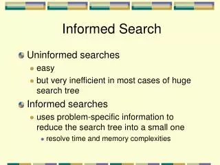
4. Zerind Sibiu Timisoara Arad Oradea Fagaras Arad Oradea Rimnicu Vilcea Lugoj Arad Breadth-first Search • Expand shallowest unexpanded node • Implementation: QueueingFn = put successors at end of queue. Arad

5. Romania with Edge Costs

6. Zerind Sibiu Timisoara 118 75 140 140 118 75 75 111 71 118 Arad Oradea Arad Lugoj 150 146 236 229 Uniform-cost Search (Dijkstra, 1959) • Let g(n) be path cost of node n. • Expand least-cost unexpanded node • Implementation: QueueingFn = insert in order of increasing path length Arad

7. Properties of Uniform-Cost Search • Complete: • Optimal: • Time: • Space: Yes if arc costs bounded below by  > 0. Yes # of nodes with g(n)  cost of optimal solution # of nodes with g(n)  cost of optimal solution Note: Breadth first is equivalent to Uniform-Cost Search with edge cost equal a constant.

8. Zerind Sibiu Timisoara Arad Oradea Timisoara Zerind Sibiu Depth-First Search • Expand deepest unexpanded node • Implementation QueueingFn = insert successors at front of queue Arad Note: Depth-first search can perform infinite cycle excursions. Need a finite, non-cyclic search space or repeated-state checking.

9. Implementation of Search Algorithms Function GENERAL-SEARCH (problem, queing-fn) returns a solution or failure queue MAKE-QUEUE (MAKE-NODE(INITIAL-STATE[problem])) loop do ifqueueis empty, then return failure node Remove-Front(queue) if GOAL-TEST [problem] applied to STATE(node) succeeds then return node ifSTATE(node) is not in closed then add STATE(node) to closed; queueQUEING-FN(queue,EXPAND(node,operators[problem])) end

10. Properties of Depth-First Search No: Fails in infinite-depth spaces, spaces with loops. Modify to avoid repeated states on path  Complete in finite spaces No O(bm): terrible if m is much larger than d. O(bm) i.e. linear in depth • Complete: • Optimal: • Time: • Space: Let b: Branching factor m: Maximum Depth

11. Iterative Deepening Search Repeated depth-limited search with increasing depth Function ITERATIVE-DEEPENING-SEARCH (problem) returns a solution or failure for depth  0 to MAXDEPTH do result  DEPTH-LIMIT-SEARCH (problem, depth) if result then return result end return FAILURE

12. Iterative Deepening Search: depth=0 Arad

13. Zerind Sibiu Timisoara Iterative Deepening Search: depth=1 Arad

14. Zerind Sibiu Timisoara Arad Oradea Fagaras Arad Oradea Rimnicu Vilcea Lugoj Arad Iterative Deepening Search: depth=2 Arad

15. Properties of Iterative Deepening Search Yes. Yes for constant edge cost. (d+1)b0 + db1 + (d-1)b2 +…+ bd =O(bd). O(bd). • Complete: • Optimal: • Time: • Space: Notes: • Maximum space is same as depth first • Time complexity is the same order as breadth first, and when branching factor is large, time is very close even with repeated searches: Example: b=10, d=5: Breadth first -> 111,111 expansions IDS -> 123,456 expansions binary trees: IDS twice as long as depth-first

16. Comparison of search Algorithms b: Branching factor d: Depth of solution m: Maximum depth l : Depth Limit

17. Informed Search Mehods

18. Best-first Search Idea: use an evaluation functionf(n) for each node -- estimate of “distance” to the goal or “path length”  Expand unexpanded node with smallest f(n) value • Implementation: QueueingFn = insert successors in increasing f(n) value • Special cases: • Uniform cost (Dijkstra’s algorithm) • Greedy search • A* search

19. Best-First Search Algorithm • Initialize Q to one-element queue consisting of the root node • While Q is not empty, do 2.a. Set N to the first element of the Q 2.b. If N is the goal node, return SUCCESS 2.c. Remove N from Q. 2.d. Add the children of N to Q, and sort the entire Queue by f(n). • Return Failure

20. Romania with Edge Costs

21. Greedy Search • Let evaluation function f(n) be an estimate of cost from node n to goal; this function is often called a heuristic and is denoted by h(n). e.g., hSLD(n) = straight-line distance from n to Bucharest • Greedy search expands the node that appears to be closest to goal. • Contrast with uniform-cost search in which lowest cost path from start is expanded.

22. Zerind 374 Sibiu 253 Timisoara 329 Rimnicu Vilcea 193 Arad 366 Oradea 380 Fagaras 178 Sibiu 253 Bucharest 0 Greedy Search Example: Arad to Bucharest Note: In this case, there wasn’t any backtracking. Arad 366

23. Properties of Greedy Search No: • Fails in infinite-depth spaces. • Spaces with loops (e.g. going from Lasi to Oradea):  Complete in finite spaces with repeated state checking. No – optimal path goes through Ptesti. O(bm): like depth first, but a good heuristic function gives dramatic improvement on average. O(bm): Potentially keeps all nodes in memory. • Complete: • Optimal: • Time: • Space: Let b: Branching factor m: Maximum Depth

24. So, why are the following optimal (find least cost path) • Breadth-first • Uniform-cost • Iterative deepening (IDS) whereas the following are not optimal? • Depth-first • Depth-limited • Greedy search

25. Answer: Stopping criterion The search procedure should stop when: The shortest incomplete path is costlier (longer) than the shortest complete path. NOT when any old path reaching the goal is found.

26. A* Search • Idea: avoid expanding paths that are already expensive • Evaluation function: f(n) = g(n) + h(n) g(n) = path cost so far to reach n. (used in uniform-cost search) h(n) = estimated path cost to goal from n. (used in greedy search) f(n) = estimated total cost of path through n to goal

27. Admissible Heuristics • A* search uses an admissible heuristic in which h(n)  h*(n) where h*(n) is the TRUE cost from n. • h(n) is a consistent underestimate of the true cost • For example, hSLD(n) never overestimates the actual road distance.

28. g(n) : cost of path h(n) : Heuristic (expected) minimum cost to goal h*(n): true minimum cost to goal Admissible Heuristics • A* search uses an admissible heuristic in which h(n)  h*(n) where h*(n) is the TRUE cost from n. root n Goal

29. 75 118 140 Zerind 449 Sibiu 393 Timisoara 447 140 99 151 80 Rimnicu Vilcea 413 Arad 646 Oradea 526 Fagaras 417 80 99 146 97 211 Craiova 526 Pitesti 415 Sibiu 553 Sibiu 591 Bucharest 450 101 97 138 Rimnicu Vilcea 607 Craiova 615 Bucharest 418 A* Search Example Arad 366

30. Proof that A* is Optimal • Let G be the optimal goal state reached by a path with cost f*=g(G). Let G2 be some other goal state or the same state, but reached by a more costly path so that g(G2)> f*. We will show that A* cannot return G2. • Let n be any unexpanded node on the shortest path to the optimal goal G. f(G2) = g(G2) since h(G2)=0 > g(G) since G2 is suboptimal  f(n) = g(n) + h(n) since h is admissible • Since f(G2) > f(n), A* will never select G2 for expansion. • !!True for trees!! • For more formal and detailed discussion/proofs than text, see: • Nilsson’s “Principles of AI” • Pearl’s “Heuristics”

31. Implementation of Search Algorithms Function GENERAL-SEARCH (problem, queing-fn) returns a solution or failure queue MAKE-QUEUE (MAKE-NODE(INITIAL-STATE[problem])) loop do ifqueueis empty, then return failure node Remove-Front(queue) if GOAL-TEST [problem] applied to STATE(node) succeeds then return node ifSTATE(node) is not in closed then add STATE(node) to closed; queueQUEING-FN(queue,EXPAND(node,operators[problem])) end

32. Consistency (= Monotonicity) • A heuristic is said to be consistent when for any node n, successor n’ of n, we have h(n) ≤ c(n,n’) + h(n’), where c(n,n’) is the (minimum) cost of a step from n to n’. • This is a form of triangular inequality: • Consistent heuristics are admissible. Not all admissible heuristics are consistent. • When a heuristic is consistent, the values of f(n) along any path are nondecreasing. • A* with a consistent heuristic is optimal. n h(n) g c(n,n’) h(n’) n’

33. A* with consistent heuristics • With consistent heuristics, A* expands nodes in order of increasing f value. • At each step, A* expands the fringe node with minimum f cost. ) The search proceeds in successive fronts (contours) of minimum f value, and the first path to any (expanded) repeated node is always the one minimizing f. ) Optimality.

34. Properties of A* Yes, even for infinite graphs unless there are infinitely many nodes with f  f(G) Yes Exponential O(bm): Potentially keeps all nodes in memory Note, A* is also optimally efficient for a given heuristic: That is, no other optimal search algorithm is guaranteed to open fewer nodes. • Complete: • Optimal: • Time: • Space: Let b: Branching factor m: Maximum Depth

35. Admissible Heuristics: Example: the 8-Puzzle 5 4 1 2 3 Goal Start 6 1 8 8 4 • Path cost: total number of vertical or horizontal moves • Two different heuristics: • h1(n) = number of misplaced tiles • h2(n) = total Manhattan distance (number of squares to desired location for each tile) So, what are h1(start) and h2(start)? h1(s) = 7 h2(s) = 2 + 3 + 3 + 2 + 4 + 2 + 0 + 2 = 18 3 7 2 7 6 5

36. Each data point corresponds to 100 instances of the 8-puzzle problem in which the solution depth varies. Dominance • Given two admissible heuristics h1(n) and h2(n), which is better? • If h’(n)  h(n) for all n, then • h’ is said to dominate h • h’ is better for search • For our 8-puzzle heuristic, does h2 dominate h1?