Understanding Instance-Based Learning: IB1, IBK, and Nearest Neighbor Techniques
This section provides a comprehensive overview of Instance-Based Learning (IBL) methods, specifically focusing on IB1 and IBK algorithms. It details the basic distance functions used to measure similarities between attribute values, including handling of real and nominal data. The text explains the concept of predicting class labels based on nearest neighbors and discusses Voronoi diagrams and voting schemes for classification. Challenges like noise, bad distance measures, and memory issues are addressed, along with solutions such as data normalization and kernel methods.

Understanding Instance-Based Learning: IB1, IBK, and Nearest Neighbor Techniques
E N D
Presentation Transcript
Instance Based Learning IB1 and IBK Small section in chapter 20
1- Nearest Neighbor • Basic distance function between attribute-values • If real, the absolute value • If nominal, d(v1,v2) = 1 if v1 \=v2, else 0. • Distance between 2 instances is square root of sum of square. • Usually normalize real-value distances for fairness amongst attributes.
Prediction • For instance x, let y be closest instance to x in training set. • Predict class x is the class of y. • On some data sets, best algorithm.
Voronoi Diagram • For each point, draw the boundary of all points closest to it. • Each point’s sphere of influence in convex. • If noisy, can be bad. • http://www.cs.cornell.edu/Info/People/chew/Delaunay.html - nice applet.
Problems and solutions • Noise • Remove bad examples • Use voting • Bad distance measure • Use probability class vector • Memory • Remove unneeded examples
Voting schemes • K nearest neighbor • Let all the closest k neighbors vote (use k odd) • Kernel K(x,y) – a similarity function • Let everyone vote, with decreasing weight according to K(x,y) • Ex: K(x,y) = e^(-distance(x,y)^2) • Ex. K(x,y) = inner product of x and y • Ex K(x,y) = inner product of f(x) and f(y) where f is some mapping of x and y into R^n.
Choosing the parameter K • Divide data into train and test • Run multiple values of k on train • Choose k that does best on test. • NOT – you have used test to data to pick the k.
Internal Cross-validation • This can be used for selecting any parameter. • Divide Data into Train and Test. • Now do 10-fold CV on the training data to determine the appropriate value of k. • Note: never touch the test data.
Probability Class Vector • Let A be an attribute with values v1, v2,..vn • Suppose class C1,C2,..Ck • Prob Class Vector for vi is: <P(C1|A=vi),P(C2|A=vi),..P(Ck|A=vi)> • Distance(vi,vj) = distance between probabiltiy class vectors.
PCV • If an attribute is irrelevant and v and v’ are values, then PCV(v) ~ PCV(v’) so the distance will be close to 0. • This discounts irrelevant attributes. • It also works for real-attributes, after binning. • Binning is a way to make real-values symbolic. Simple break data into k bins, eg. K = 5 or 10 seems to work. Or use DTs.
Regression by NN • If 1-NN, use value of nearest example • If k-nn, interpolate values of k nearest neighbors. • Kernel methods work to. You avoid choice of k, but hide it in choice of kernel function.
Summary • NN works for multi-class and regression. • Sometimes called “poor man’s neural net’’ • With enough data, it achieves ½ the “bayes optimal” error rate. • Mislead by bad examples and bad features. • Separates classes via piecewise linear boundaries.