Instance Based Learning
Instance Based Learning. Based on Raymond J. Mooney’s slides University of Texas at Austin. Example. Instance-Based Learning.


Instance Based Learning
E N D
Presentation Transcript
Instance Based Learning Based on Raymond J. Mooney’s slides University of Texas at Austin
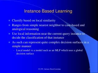
Instance-Based Learning • Unlike other learning algorithms, does not involve construction of an explicit abstract generalization but classifies new instances based on direct comparison and similarity to known training instances. • Training can be very easy, just memorizing training instances. • Testing can be very expensive, requiring detailed comparison to all past training instances. • Also known as: • Case-based • Exemplar-based • Nearest Neighbor • Memory-based • Lazy Learning
Similarity/Distance Metrics • Instance-based methods assume a function for determining the similarity or distance between any two instances. • For continuous feature vectors, Euclidian distance is the generic choice: Where ap(x) is the value of the p th feature of instance x. • For discrete features, assume distance between two values is 0 if they are the same and 1 if they are different (e.g. Hamming distance for bit vectors). • To compensate for difference in units across features, scale all continuous values to the interval [0,1].
Other Distance Metrics • Mahalanobis distance () • Scale-invariant metric that normalizes for variance. • Cosine Similarity • Cosine of the angle between the two vectors. • Used in text and other high-dimensional data. • Pearson correlation () • Standard statistical correlation coefficient. • Edit distance • Used to measure distance between unbounded length strings.
K-Nearest Neighbor • Calculate the distance between a test point and every training instance. • Pick the k closest training examples and assign the test instance to the most common category amongst these nearest neighbors. • Voting multiple neighbors helps decrease susceptibility to noise. • Usually use odd value for k to avoid ties.
Implicit Classification Function • Although it is not necessary to explicitly calculate it, the learned classification rule is based on regions of the feature space closest to each training example. • For 1-nearest neighbor with Euclidian distance, the Voronoi diagram gives the complex polyhedra segmenting the space into the regions closest to each point.
Efficient Indexing • Linear search to find the nearest neighbors is not efficient for large training sets. • Indexing structures can be built to speed testing. • For Euclidian distance, a kd-tree can be built that reduces the expected time to find the nearest neighbor to O(log n) in the number of training examples. • Nodes branch on threshold tests on individual features and leaves terminate at nearest neighbors. • Other indexing structures possible for other metrics or string data. • Inverted index for text retrieval.
kd-tree • The kd-tree is a binary tree in which every node is a k-dimensional point. • Every non-leaf node generates a splitting hyperplane that divides the space into two subspaces. • Points left to the hyperplane represent the left sub-tree of that node and the points right to the hyperplane by the right sub-tree. • The hyperplane direction is chosen in the following way: every node split to sub-trees is associated with one of the k-dimensions, such that the hyperplane is perpendicular to that dimension vector.
Nearest Neighbor Variations • Can be used to estimate the value of a real-valued function – regression - by taking the average function value of the k nearest neighbors to an input point. • All training examples can be used to help classify a test instance by giving every training example a vote that is weighted by the inverse square of its distance from the test instance.
Feature Relevance and Weighting • Standard distance metrics weight each feature equally when determining similarity. • Problematic if many features are irrelevant, since similarity along many irrelevant examples could mislead the classification. • Features can be weighted by some measure that indicates their ability to discriminate the category of an example, such as information gain. • Overall, instance-based methods favor global similarity over concept simplicity.
Rules and Instances inHuman Learning Biases • Psychological experiments show that people from different cultures exhibit distinct categorization biases. • “Western” subjects favor simple rules (straight stem) and classify the target object in group 2. • “Asian” subjects favor global similarity and classify the target object in group 1.
Other Issues • Can reduce storage of training instances to a small set of representative examples. • Support vectors in an SVM are somewhat analogous. • Can hybridize with rule-based methods or neural-net methods. • Radial basis functions in neural nets and Gaussian kernels in SVMs are similar. • Can be used for more complex relational or graph data. • Similarity computation is complex since it involves some sort of graph isomorphism. • Can be used in problems other than classification. • Case-based planning • Case-based reasoning in law and business.
Conclusions • IBL methods classify test instances based on similarity to specific training instances rather than forming explicit generalizations. • Typically trade decreased training time for increased testing time.
Clustering Partition unlabeled examples into disjoint subsets of clusters, such that: Examples within a cluster are very similar Examples in different clusters are very different Discover new categories in an unsupervised manner (no sample category labels provided). 16
Clustering Example . . . . . . . . . . . . . . . . . . . . . . . . . . . . . . . . 17
Hierarchical Clustering Build a tree-based hierarchical taxonomy (dendrogram) from a set of unlabeled examples. Recursive application of a standard clustering algorithm can produce a hierarchical clustering. animal vertebrate invertebrate fish reptile amphib. mammal worm insect crustacean 18
Aglommerative vs. Divisive Clustering Aglommerative (bottom-up) methods start with each example in its own cluster and iteratively combine them to form larger and larger clusters. Divisive (partitional, top-down) separate all examples immediately into clusters. 19
Direct Clustering Method Direct clustering methods require a specification of the number of clusters, k, desired. A clustering evaluationfunctionassigns a real-value quality measure to a clustering. The number of clusters can be determined automatically by explicitly generating clusterings for multiple values of k and choosing the best result according to a clustering evaluation function. 20
Hierarchical Agglomerative Clustering (HAC) Assumes a similarity function for determining the similarity of two instances. Starts with all instances in a separate cluster and then repeatedly joins the two clusters that are most similar until there is only one cluster. The history of merging forms a binary tree or hierarchy. 21
HAC Algorithm Start with all instances in their own cluster. Until there is only one cluster: Among the current clusters, determine the two clusters, ci and cj, that are most similar. Replace ci and cj with a single cluster ci cj 22
Cluster Similarity Assume a similarity function that determines the similarity of two instances: sim(x,y). Euclidean /Mahalanobis, Hamming, Cosine similarity, Pearson r etc. How to compute similarity of two clusters each possibly containing multiple instances? Single Link: Similarity of two most similar members. Complete Link: Similarity of two least similar members. Group Average: Average similarity between members. 23
Single Link Agglomerative Clustering Use maximum similarity of pairs: Can result in “straggly” (long and thin) clusters due to chaining effect. Appropriate in some domains, such as clustering islands. 24
Complete Link Agglomerative Clustering Use minimum similarity of pairs: Makes more “tight,” spherical clusters that are typically preferable. 26
Computational Complexity In the first iteration, all HAC methods need to compute similarity of all pairs of n individual instances which is O(n2). In each of the subsequent n2 merging iterations, it must compute the distance between the most recently created cluster and all other existing clusters. In order to maintain an overall O(n2) performance, computing similarity to each other cluster must be done in constant time. 28
Computing Cluster Similarity After merging ci and cj, the similarity of the resulting cluster to any other cluster, ck, can be computed by: Single Link: Complete Link: 29
Group Average Agglomerative Clustering Use average similarity across all pairs within the merged cluster to measure the similarity of two clusters. Compromise between single and complete link. Averaged across all ordered pairs in the merged cluster instead of unordered pairs between the two clusters to encourage tight clusters. 30
Computing Group Average Similarity Assume cosine similarity and normalized vectors with unit length. Always maintain sum of vectors in each cluster. Compute similarity of clusters in constant time: 31
Non-Hierarchical Clustering Typically must provide the number of desired clusters, k. Randomly choose k instances as seeds, one per cluster. Form initial clusters based on these seeds. Iterate, repeatedly reallocating instances to different clusters to improve the overall clustering. Stop when clustering converges or after a fixed number of iterations. 32
K-Means Assumes instances are real-valued vectors. Clusters based on centroids, center of gravity, or mean of points in a cluster, c: Reassignment of instances to clusters is based on distance to the current cluster centroids. 33
Distance Metrics Euclidian distance (L2 norm): L1 norm: Cosine Similarity (transform to a distance by subtracting from 1): 34
K-Means Algorithm Let d be the distance measure between instances. Select k random instances {s1, s2,… sk} as seeds. Until clustering converges or other stopping criterion: For each instance xi: Assign xi to the cluster cjsuch that d(xi, sj) is minimal. (Update the seeds to the centroid of each cluster) For each cluster cj sj = (cj) 35
K Means Example(K=2) Pick seeds Reassign clusters Compute centroids Reasssign clusters x x x Compute centroids x x x Reassign clusters Converged! 36
Time Complexity Assume computing distance between two instances is O(m) where m is the dimensionality of the vectors. Reassigning clusters: O(kn) distance computations, or O(knm). Computing centroids: Each instance vector gets added once to some centroid: O(nm). Assume these two steps are each done once for I iterations: O(Iknm). Linear in all relevant factors, assuming a fixed number of iterations, more efficient than O(n2) HAC. 37
K-Means Objective The objective of k-means is to minimize the total sum of the squared distance of every point to its corresponding cluster centroid. • Finding the global optimum is NP-hard. • The k-means algorithm is guaranteed to converge a local optimum. 38
Seed Choice Results can vary based on random seed selection. Some seeds can result in poor convergence rate, or convergence to sub-optimal clusterings. Select good seeds using a heuristic or the results of another method. 39
Buckshot Algorithm Combines HAC and K-Means clustering. First randomly take a sample of instances of size n Run group-average HAC on this sample, which takes only O(n) time. Use the results of HAC as initial seeds for K-means. Overall algorithm is O(n) and avoids problems of bad seed selection. 40
Text Clustering HAC and K-Means have been applied to text in a straightforward way. Typically use normalized, TF/IDF-weighted vectors and cosine similarity. Optimize computations for sparse vectors. Applications: During retrieval, add other documents in the same cluster as the initial retrieved documents to improve recall. Clustering of results of retrieval to present more organized results to the user à la Northernlight folders (). Automated production of hierarchical taxonomies of documents for browsing purposes (à la Yahoo & DMOZ). 41
Soft Clustering Clustering typically assumes that each instance is given a “hard” assignment to exactly one cluster. Does not allow uncertainty in class membership or for an instance to belong to more than one cluster. Soft clustering gives probabilities that an instance belongs to each of a set of clusters. Each instance is assigned a probability distribution across a set of discovered categories (probabilities of all categories must sum to 1). 42
Expectation Maximumization (EM) Probabilistic method for soft clustering. Direct method that assumes k clusters:{c1, c2,… ck} Soft version of k-means. Assumes a probabilistic model of categories that allows computing P(ci | E)for each category, ci, for a given example, E. For text, typically assume a naïve-Bayes category model. Parameters = {P(ci), P(wj | ci): i{1,…k}, j {1,…,|V|}} 43
EM Algorithm Iterative method for learning probabilistic categorization model from unsupervised data. Initially assume random assignment of examples to categories. Learn an initial probabilistic model by estimating model parameters from this randomly labeled data. Iterate following two steps until convergence: Expectation (E-step): Compute P(ci | E)for each example given the current model, and probabilistically re-label the examples based on these posterior probability estimates. Maximization (M-step): Re-estimate the model parameters, , from the probabilistically re-labeled data. 44
EM + + + + + Initialize: Assign random probabilistic labels to unlabeled data Unlabeled Examples 45
EM Prob. Learner + + + + + Initialize: Give soft-labeled training data to a probabilistic learner 46
EM Prob. Learner Prob. Classifier + + + + + Initialize: Produce a probabilistic classifier 47
EM Prob. Learner Prob. Classifier + + + + + E Step: Relabel unlabled data using the trained classifier 48
EM Prob. Learner Prob. Classifier + + + + + M step: Retrain classifier on relabeled data Continue EM iterations until probabilistic labels on unlabeled data converge. 49
Learning from Probabilistically Labeled Data Instead of training data labeled with “hard” category labels, training data is labeled with “soft” probabilistic category labels. When estimating model parameters from training data, weight counts by the corresponding probability of the given category label. For example, if P(c1 | E) = 0.8 and P(c2 | E) = 0.2, each word wj in E contributes only 0.8 towards the counts n1 and n1j, and 0.2 towards the counts n2 and n2j . 50