Instance Based Learning
Instance Based Learning. Introduction k-nearest neighbor Locally weighted regression Radial Basis Functions Case-Based Reasoning Summary. Introduction. Instance-based learning divides into two simple steps: 1. Store all examples in the training set.

Instance Based Learning
E N D
Presentation Transcript
Instance Based Learning • Introduction • k-nearest neighbor • Locally weighted regression • Radial Basis Functions • Case-Based Reasoning • Summary
Introduction Instance-based learning divides into two simple steps: 1. Store all examples in the training set. 2. When a new example arrives, retrieve those examples similar to the new example and look at their classes. • Disadvantages: • Classification cost may be high; why? (we look for efficient indexing techniques). • Irrelevant attributes may increase the distance of “truly” similar examples.
K-nearest neighbor To define how similar two examples are we need a metric. We assume all examples are points in an n-dimensional space Rn and use the Euclidean distance: Let Xi and Xj be two examples. Their distance d(Xi,Xj) is defined as d(Xi, Xj) = Σk [xik – xjk]2 Where xik is the value of attribute k on example Xi.
K-nearest neighbor for discrete classes Example: New example K = 4
Voronoi Diagram Decision surface induced by a 1-nearest neighbor. The decision surface is a combination of convex polyhedra surrounding each training example.
K-nearest neighbor for discrete classes Algorithm (parameter k) 1. For each training example (X,C(X)) add the example to our training list. 2. When a new example Xq arrives, assign class: C(Xq) = majority voting on the k nearest neighbors of Xq C(Xq) = argmax v Σi δ(v, C(Xi)) where δ(a,b) = 1 if a = b and 0 otherwise
K-nearest neighbor for real-valued functions Algorithm (parameter k) 1. For each training example (X,C(X)) add the example to our training list. 2. When a new example Xq arrives, assign class: C(Xq) = average value among k nearest neighbors of Xq C(Xq) = Σ C(Xi) / k
Distance Weighted Nearest Neighbor It makes sense to weight the contribution of each example according to the distance to the new query example. C(Xq) = argmax v Σi wi δ(v, C(Xi)) For example, wi = 1 / d(Xq,Xi)
Distance Weighted Nearest Neighborfor Real-Valued Functions For real valued functions we average based on the weight function and normalize using the sum of all weights. C(Xq) = Σi wi C(Xi) / Σ wi
Problems with k-nearest Neighbor • The distance between examples is based on all attributes. What if some attributes are irrelevant? • Consider the curse of dimensionality. • The larger the number of irrelevant attributes, the higher the effect on the nearest-neighbor rule. One solution is to use weights on the attributes. This is like stretching or contracting the dimensions on the input space. Ideally we would like to eliminate all irrelevant attributes.
Locally Weighted Regression Let’s remember some terminology: Regression.- Is a problem similar to classification but the value to predict is a real number. Residual.- The difference between the true target value f and our approximation f’: f(X) – f’(X) Kernel Function.- The distance function that provides a weight to each example. The kernel function K is a function of the distance between examples: K = f(d(Xi,Xq))
Locally Weighted Regression • The method is called locally weighted regression for the • following reasons: • “Locally” because the predicted value for an example Xq • is based only on the vicinity or neighborhood around Xq. • “Weighted” because the contribution of each neighbor of • Xq will depend on the distance between the neighbor • example and Xq. • “Regression” because the value to predict will be a real • number.
Locally Weighted Regression Consider the problem of approximating a target function using a linear combination of attribute values: f’(X) = w0 + w1x1 + w2x2 + … + wnxn Where X = (x1, x2, …, xn) We want to find those coefficients that minimize the error: E = ½ Σk [f(X) – f’(X)]2
Locally Weighted Regression If we do this in the vicinity of an example Xq and we wish to use a kernel function, we get a form of locally weighted regression: E(Xq) = ½ Σk ( [f(X) – f’(X)]2 K(d(Xq,X) ) Where the sum now goes over the neighbors of Xq.
Locally Weighted Regression Using gradient descent search, the update rule is defined as: Δ Wj = n Σk [f(X) – f’(X)]K(d(Xq,X) xj where n is the learning rate and xj is the jth attribute of example X.
Locally Weighted Regression • Remarks: • The literature contains other functions that are non linear. • There are many variations to locally weighted regression that use different kernel functions. • Normally a linear model is sufficiently good to approximate the local neighborhood of an example.