Download
1 / 20
210 likes | 344 Views
Explore a new model for visual analysis of graph structures with magnetic force emitters and color-coded interactions. This doctoral study from Riga Technical University presents innovative visualization techniques and layout algorithms. Discover how force-based approaches and precise color distinctions improve graph representation. The magnetic force emitters enable dynamic control for enhanced user interaction.

E N D
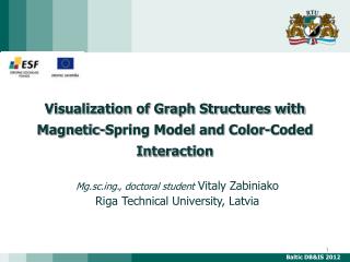
Visualization of Graph Structures with Magnetic-Spring Model and Color-Coded Interaction Mg.sc.ing., doctoral studentVitaly Zabiniako Riga Technical University, Latvia Baltic DB&IS 2012
Problem domain (1/4) Simplicity and complexity of visual data: Formalization: Simple Complex Graph Baltic DB&IS 2012
Problem domain (2/4) Application: • Organizational charts • Web site maps • Data structures • Semantic networks • State–transition diagrams • Object–oriented systems • (class browsers) • Petri nets • Data flow diagrams • Subroutine–call graphs • Entity relationship diagrams • Knowledge–representation • diagrams • Taxonomies • Project/document • management systems • Evolutionary trees • Molecular maps • in biology and chemistry Baltic DB&IS 2012
Problem domain (3/4) Visualization of graphs • Graph layout algorithms • Visualization • techniques • Usage of two-dimensional / • three-dimensional space • GVS (Graph • Visualization Systems) Baltic DB&IS 2012
Problem domain (4/4) • preliminary visual analysis before automatic processing; • B. Schneiderman – “Overview first, zoom and filter, then details on demand”. …a model for improved data analysis and interaction! Baltic DB&IS 2012
Goal and tasks • Goal: • to improve capabilities of visual analysis of graph structures by providing a new model for interaction between the user and GVS. Tasks: • to analyze aspects of existing graph layout models; • to introduce a concept of MFE (Magnetic Force Emitter) and its interaction rules, based on the RGB / HSL color models; • to provide a specification of an integrated virtual workshop for graph visualization; • to demonstrate the proposed approach in a case-study. Baltic DB&IS 2012
Force-based approach (1/3) Peter Eades – “A heuristic for graph drawing”, 1984. • Forces of attraction and repulsion: • Average kinetic energy: /*1*/ place vertices of G in random locations; /*2*/ repeat until equilibrium /*3*/ calculate the force on each vertex; /*4*/ move the vertex (force on vertex) /*5*/ draw graph • Algorithm: • Result: Baltic DB&IS 2012
Force-based approach (2/3) Kozo Sugiyama – “A Simple and Unified Method for Drawing Graphs: Magnetic-Spring Algorithm”, 1994. + • Magnetic fields: • parallel; • polar; • concentric; • compound orthogonal; • compound polar-concentric. Baltic DB&IS 2012
Force-based approach (3/3) • Explicit benefits: • outlining of geometrically localized subsets (clusters) of elements with dense mutual relations • keeping decoupled clusters separate; • outlining of symmetric structures (if any) within the graph; • reduced bounding box (minimization of occupied space); • Implicit benefits: • dynamic evolving; • altering with additional force fields. • Drawbacks: • computational complexity; • avoiding local minima of . Baltic DB&IS 2012
Magnetic Force Emitters • to allow for MFE the conditional stop is removed from the algorithm. This: • leaves the virtual model of a graph in permanent “standby” state • and • enables reactions to additional dynamic force emitters which are positioned and controlled by the user in virtual visualization space. • eg. “auto-attract”and localize nodes which conforms to user-defined criteria(only inherited classes in UML diagram, only non-empty folders in file system, etc.); • “auto-repulse” nodes which must be filtered out of the inspection, etc. Baltic DB&IS 2012
Color-coded interaction (1/4) • concept of a color is well-known and implicitly understandable by most humans; • according formalized models exist , known as RGB / HSL color spaces: • RGB relies on Cartesian coordinate system and distance between colors; • HSL is based on cylindrical coordinate system; • “equal”/“close”, “separate”/“opposite” colors, e.g.: [blue, yellow]; [red, cyan]; [green, magenta]; [black, white] (opposite vertices in RGB / separation by angle π in HSL). Baltic DB&IS 2012
Color-coded interaction (2/4) • visual interaction rules between arbitrary graph element E (RE,GE,BE) and magnetic force emitter M (RM,GM,BM) define force modifier function f for attraction / repulsion: • Fa’= Fa ∙ f(RE,GE,BE,RM,GM,BM) • Fr’= Fr ∙ f(RE,GE,BE,RM,GM,BM) • RGB: • color-based contradistinction • f(RE,GE,BE,RM,GM,BM) = DRGB • color-based proximity f(RE,GE,BE,RM,GM,BM) = (1–DRGB) Baltic DB&IS 2012
Color-coded interaction (3/4) • HSL: • color-based contradistinction • f(RE,GE,BE,RM,GM,BM) = DHSL • color-based proximity f(RE,GE,BE,RM,GM,BM) = (1–DHSL) Baltic DB&IS 2012
Color-coded interaction (4/4) • RGB: • equal colors results in DRGB = 0, while “opposite” colors have DRGB = 1; • visually similar colors have DRGB which usually does not exceed 0.4; • all primary colors have distinctive mutual normalized distances; • grey color is equally “close”/”apart” from all other primary colors. • HSL: • equal colors results in DHSL=0, while “opposite” colors have DHSL=1; • visually similar colors tend to have smaller DHSL; • all primary colors have distinctive mutual normalized distances; • black, white and all shades of grey color cannot participate in interaction (arctan2 is undefined); • has better distribution due to the fact that visually close colors have smaller values (as an example: (1,0,1) – (0.69, 0.2, 0.96) has DHSL=0,11 versus DRGB = 0,21; (0,0,1) – (0.29,0.39,0.85) has DHSL=0,05 versus DRGB = 0,3, etc). Baltic DB&IS 2012
A concept of virtual workshop Within the scene (1) there is inner virtual frustum (2) which defines borders of the “workshop”. Within the inner frustum the spatial graph model is situated. Its elements can be manipulated with the help of MFE (6) by attracting / repulsing color-compatible elements (5). Faces of the inner frustum might be used as magnetic planes (7) which attract compatible nodes (4) while the remaining graph elements (3) stay on the background. Baltic DB&IS 2012
A case study of color-coded interaction • A topological model for library application: • initial graph (1); • application of unmodified force-based layout (2); • introduction of “green” MFE (3); • visual distinction of “yellow” cycle via front magnetic plane (4). Baltic DB&IS 2012
Conclusions (1/2) • A novel approach for visualization of graphs, based on dynamic color-coded interaction and magnetic-spring model is presented. • An attempt was made to unite two consistent approaches (physical phenomenon of magnetic interaction and color vision) both of which exist in a real world, and apply these to the information visualization domain. • The RGB color distance is valid for all possible color combinations, while having average precision for identifying visually “close” colors.
Conclusions (2/2) • The HSL color distance features better convergence, although it is not capable of working with monochrome colors. • Both strategies are compatible with proposed concept of virtual workshop which relies on frustum space, manipulation with MFE, magnetic planes and auxiliary layout algorithms / visualization techniques. • Implementation details of how the color of graph elements is being defined, how the user controls MFE and defines color of these must be solved during implementation of particular GVS.
Future development • Exploration of additional color-based interaction • models (CIELAB, etc.); • rules; • Elaboration of standardized recommendations for manipulation of properties of MFE and frustum planes. • Adapting additional visualization techniques for better information comprehension within integrated virtual workshop of GVS.
Thank you for attention! Any questions…?