Download
1 / 44
440 likes | 555 Views
Explore how to find z-scores when given probabilities under any normal curve, determining acceptance thresholds based on z-scores, and applying z-scores in real-world scenarios such as employee retention decisions.

E N D
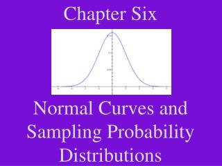
Chapter SixNormal Curves and Sampling Probability Distributions
Chapter 6 Section 3 Areas Under Any Normal Curve
Finding Z Scores When Probabilities (Areas) Are Given Find the indicated z score: if P(0 < z < zcutoff) = 0.3907 0.3907 P(0 < z < 1.23) .3907 0 z = ? z = 1.23
Find the indicated z score:if P(zcutoff < z < 0) = 0.1331 0.1331 P(-0.34 < z < 0) 0.1331 ? = z0 z = –0.34
Find the indicated z score:if P(z < zcutoff) = 0.8554 0.8554 0.5000+0.3554 P(z < 1.06) 0.8554-0.5000 0.3554 .8554 0 z = ? z = 1.06
Find the indicated z score:if P(z < zcutoff) = 0.0681 0.06810.5000 - 0.4319P(z < -1.49) 0.5000-0.0681 0.4319 0.0681 z 0 z = -1.49
Find the indicated z score:if P(z > zcutoff) = 0.01 0.010.5000 - 0.4900P(z > 2.33) 0.5000- .0100 0.4900 .01 z 0 z = 2.33
Find the indicated z score:if P(z < zcutoff) = 0.005 0.0050 0.5000 - 0.4950 P(z < – 2.575) 0.5000-0.0050 .4950 .005 0 z z = – 2.575
Find the indicated z score:if 1% is in the tail regions Area A + Area B = .01andArea A = Area B So, Area A = 0.005and Area B = 0.005 0.012(0.005)2(0.5000 - 0.4950)P (z < -2.575) or P(z > 2.575) 1.0000 - 0.01000.99000.4950 + 0.4950 B A .4950 .4950 – z 0 z z = -2.575 z = 2.575
Find the indicated z score: if 5% is in the tail regions Area A + Area B = .05andArea A = Area B So, Area A = 0.025and Area B = 0.025 0.052(0.025)2(0.5000 - 0.4750)P (z < -1.96) or P(z > 1.96) 1.0000 - 0.05000.95000.4750 + 0.4750 A B .4750 .4750 – z 0 z z = -1.96 z = 1.96
Application of Determining z Scores The Verbal SAT test has a mean score of 500 and a standard deviation of 100. The scores are normally distributed. A major university determines that it will accept only students whose Verbal SAT scores are in the top 4%. What is the minimum score that a student must earn to be accepted?
Application of Determining z Scores The cut-off score is 1.75 standard deviations above the mean. 0.0400 0.4600 0 z z = 1.75 Students would need to score 675 or above.
Application of Determining z Scores The length of time employees have been working at a specific company is normally distributed with a mean of 15 years and a standard deviation of 5.2 years. The CEO has decided due the recent hard economic times that the work force must be reduced by 5%. He decided to offer a retirement incentive for the longest working employees and to lay off a portion of the most recently hired employees. If he is able to split the percentage evenly between the two groups, what is his target range for the years of employment?
Application of Determining z Scores 0.0500 2(0.0250) 2(0.5000-0.4750) The cut-off score is ±1.96 standard deviations. 0.4750 0.4750 -z 0 z 0.0250 0.0250 z = 1.96 z = -1.96
Application of Determining z Scores The CEO should offer the retirement package to those employees that have worked at the company for over 25.1920 years and he must layoff employees that have worked for the company less than 4.8080 years.
Introduction Packet Questions
1. If x is a normally distributed variable with a mean of 30 and a standard deviation of 6, find the following probabilities: \ 0.00
1. If x is a normally distributed variable with a mean of 30 and a standard deviation of 6, find the following probabilities: 1.00
1. If x is a normally distributed variable with a mean of 30 and a standard deviation of 6, find the following probabilities: -2.00
1. If x is a normally distributed variable with a mean of 30 and a standard deviation of 6, find the following probabilities: -1.00 1.50
2. Determine the z scores that produce the following probabilities. a. 0.20 lies to the right of the z-score 0.84
2. Determine the z scores that produce the following probabilities. b. 0.40 lies to the right of the z-score 0.25
2. Determine the z scores that produce the following probabilities. c. 0.875 lies to the right of the z score. -1.15
2. Determine the z scores that produce the following probabilities. d. 0.6328 lies between z and -z. -0.90 0.90
3. Consider the following data set: to answer the following questions. a. Make a histogram for this data
3. Consider the following data set: to answer the following questions. b. Make a Box-n-Whisker plot for the data. <----+----+----+----+----+----+----+----+----+----> 0 1 2 3 4 5 6 7 8
3. Consider the following data set: to answer the following questions. c. What is the Pearson’s Index for the set of data?
3. Consider the following data set: to answer the following questions. d. Make a normal quantile plot for the data.
3. Consider the following data set: to answer the following questions. e. Interpret the results from parts a through d. The data appears to be normally distributed since: 1. The histogram seems to roughly fit the bell-shaped curve. 2. The Box-n-Whiskers plot does not have any outliers and appears symmetrical. 3. The Pearson’s Index of Skewness is in the normal range of -1 < PI < 1 since PI = 0.2400. 4. The Normal Quantile Plot (Normal Probability Plot) produces a graph where the data points lie in a relatively close line.
Homework Assignments Pages 286 - 291 Exercises: 1, 5, 9, 13, 17, 21, 25, 29, 33, and 37 Exercises: 3, 7, 11, 15, 19, 23, 27, 31, 35, and 39 Exercises: 2, 6, 10, 14, 18, 22, 26, 30, 34, and 38 Exercises: 4, 8, 12, 16, 20, 24, 28, 32, 36, and 40