GPS Data Integration
590 likes | 612 Views
This module will guide you through the process of importing, differentially correcting, and exporting GPS data into an ESRI-compatible format for integration into ArcView 8. Learn how to reduce positional errors and ensure the longevity of your data sets through metadata creation and projection information.

GPS Data Integration
E N D
Presentation Transcript
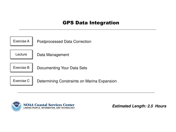
Lecture Exercise A Data Management Postprocessed Data Correction Exercise B Exercise C Documenting Your Data Sets Determining Constraints on Marina Expansion GPS Data Integration Estimated Length: 2.5 Hours
Before collected GPS data can be used, they must undergo certain process steps to successfully integrate them into a GIS. Differentially correcting and exporting the data into ESRI shapefile format will ensure that you will be able to integrate the data into ArcGIS in the short term, but what about future users of the data sets? A fully developed metadata record and projection information for your data will complete the integration process and give longevity to the data sets. The lecture and exercises in this module will guide you through the GPS data integration process. The final exercise will use the collected data sets to determine constraints on marina expansion at the data collection site. Differential correction of collected GPS data Metadata creation in ArcCatalog Setting projection information in ArcToolbox GPS Data Integration Module Introduction Overview • Software • Trimble Pathfinder Office 2.90 • ArcGIS 8.3 • ArcGIS Components • ArcMap • ArcCatalog • ArcToolbox • Geoprocessing Tools • Select-By-Attributes • Select-By-Location Tools and Technology Skills Learned
Background You have successfully created a data collection plan and used it to collect spatial features in the field using GPS, but your work is not quite over yet. Recall that even with selective availability turned off, your GPS data could still have positional errors of around 10 meters or greater. Your field data collection Statement of Work (SOW) states that differential correction be used to reduce positional errors down to one to three meters. In this exercise, you will import the uncorrected GPS data from the field activity, differentially correct it, and export it using Trimble Pathfinder Office. Objectives Import data from Trimble units Differentially correct data using post-processed method Export data into ESRI shapefile format GPS Data Integration Exercise A: Postprocessed Data Correction Goal After completing the exercise, the student will be able to successfully import, differentially correct, and export collected data into an ESRI-compatible format for integration into ArcView 8.
GPS Data Integration Exercise A: Postprocessed Data Correction • Trimble Pathfinder Office 2.90 • Differential Correction Module • Export Module Tools to Use • Summary of Process Steps • Differentially Correct GPS Data – Download a National Geodetic Survey (NGS) continuously operating reference station (CORS) correction file and use post-processed differential correction to remove errors from collected data • Use ShapeCorrect to apply corrections – Apply differential corrections to shapefiles Data Data used in this exercise will include *.ssf – uncorrected spatial data set from Trimble unit *.cor – corrected spatial data set
GPS Data Integration Exercise A: Postprocessed Data Correction • In addition to retrieving base files through Pathfinder Office, you can also download base station correction files through a Web browser. Navigate to • www.ngs.noaa.gov/CORS/ Did You Know? • 1. Differentially correct GPS data • Open Pathfinder Office. Click on Utilities > Differential Correction. • The rover file that you collected this morning should be listed in the selected files dialog; if it is not, click on the Browse button and manually select it (your instructor will provide the location of the downloaded file). • In this exercise, you will use Pathfinder Office to obtain a base file from the Internet (see sidebar for details on an alternative method for retrieving base files). • In the Base Files dialog, click on the Internet Search button. On the Internet Search window, click on the New button. Next, choose to select the new base station provider from the current list and Click OK. Select CORS, Charleston SC from the base provider list and click OK. • Sometimes the nearest base station isn’t available and you must choose another. What is the maximum distance you could have between you and the nearest available base station? ________________________________________________________________ • With the CORS, Charleston SC base station provider highlighted, click OK on the Internet Search window. Click Yes on the next window to allow the program to search the Internet through the Center’s Local Area Network (LAN) connection.
GPS Data Integration Exercise A: Postprocessed Data Correction • It may be possible to collect data when satellite positional quality is poor (i.e., high PDOP and low number of satellites available), but you may not be able to correct your data afterwards. Remember that base stations would be subject to the same poor satellite conditions as your receiver and may not be able to get reliable positional determination. • In this situation, corrections are not calculated and you would get no base file coverage. It pays to plan out your data collection activity! Did You Know? • 1. Differentially correct GPS data (continued) • After the program has finished obtaining the base files from the Internet, a confirmation window will appear. This window will list the rover data file as well as the base file and the data collection times for each . The most important item to note is the % coverage of the base file’s corrections with the rover file. Ideally, you want this value to be as close to 100% as possible. Click OK twice to apply the base file. • But what if the % coverage is significantly lower? This could be caused by a conflict between the collection times of the two files. If you started collecting data at 9:07 a.m., finished at 10:21, and downloaded corrections at 10:40, the coverage will be lower because the base station has not finished collecting data for the time period between 10 and 11 a.m.. To increase the coverage, download base data sometime after 11:00. • Leave the corrected file’s output location and file extension as their defaults. Changing either of these values could cause some difficulty in locating the corrected file. • Click OK to differentially correct your data and Close once the operation has finished.
GPS Data Integration Exercise A: Postprocessed Data Correction • If you didn’t use ShapeCorrect to correct your shapefiles, their positions would have a horizontal positional error of at least 10 meters! When in doubt, always differentially correct your data. Did You Know? • 2. Use ShapeCorrect to apply corrections • In the Windows Start Menu, navigate to Program Files > GPS Pathfinder Office 2.90 > ShapeCorrect. • You will notice that all of the shapefiles that you collected should appear in the Selected files dialog at the top of the window. If this is not the case, click on the Browse button and navigate to the location of the shapefiles (c:\Student\GPS_Data) • Next, choose to output only corrected positions, and click OK. • ShapeCorrect will read your *.cor correction file from the differential correction process and apply any necessary corrections in the x,y, and z to your shapefile coordinates. The result is a shapefile with positions that are accurate to 1 to 3 meters in the horizontal. END OF EXERCISE A
GPS Data Integration Exercise A: Postprocessed Data Correction • 3. Export data from Pathfinder Office (continued) p. 7 The maximum distance that you could have between yourself and the nearest base station is between 150 and 200 kilometers. Performing differential correction is crucial to ensuring that your data is as accurate as possible. In this exercise you used post-processing to correct your data, minimizing errors from tens of meters down to between one and three meters. Even though you have exported your data into an ArcView shapefile format, you have not finished integrating your GPS data sets into a GIS. The next lecture and following exercise will help you complete the process. Exercise Summary Answers to Exercise Questions
What do you need to document about your files for someone to be able to use these files without you? How would you capture this information? ___________________________________________________________________ ___________________________________________________________________ ___________________________________________________________________ ___________________________________________________________________ ___________________________________________________________________ ___________________________________________________________________ ___________________________________________________________________ ___________________________________________________________________ ___________________________________________________________________ ___________________________________________________________________ ___________________________________________________________________ ___________________________________________________________________ GPS Data Integration Discussion: Data Documentation
GPS Data Integration Lecture: Data Management • Documenting Your Data • Data may be in ArcGIS format, but… • What are the projection parameters? • How were the data collected? • Have the data been modified? • Two things can be done to ensure that future users will be able to answer these questions: • METADATA, METADATA, METADATA!!! • Set the projection and create a .prj file in ArcToolbox How can I use this data if I don’t know anything about it ??!!
GPS Data Integration Lecture: Data Management • Metadata in ArcCatalog • Simple to create: • Projection parameters automatically captured (if .prj file present) • Can use template to automatically fill in contact, distribution information • When documenting GPS data, be sure to include detailed process step information • Include type of correction, date, and time if not captured in attributes • Known sources of error at location?
GPS Data Integration Lecture: Data Management • Metadata in ArcCatalog • Allows you to create, view, or store metadata in variety of formats: • Federal Geographic Data Committee (FGDC) • ESRI • International Organization for Standardization (ISO) • Allows you to edit your metadata in two ways: • ISO Wizard • FGDC Editor FGDC Editor ISO Wizard
GPS Data Integration Lecture: Data Management Stylesheets FDGC Classic ISO ESRI FDGC XML
GPS Data Integration Lecture: Data Management • Importing Metadata • You can import metadata you created outside of ArcGIS using the Importer • You can also import metadata templates you have created • ArcCatalog can automatically update some fields • You can create your own importers to bring in custom metadata Warning: Importing Metadata Will Overwrite any Existing Metadata!!!
GPS Data Integration Lecture: Data Management • Exporting Metadata • You can export your metadata for use in other applications in HTML or XML format • You can also use the FGDC CSDGM Exporter to export your metadata into various formats including text • This exporter will also filter out any non-FGDC-required data for you
GPS Data Integration Lecture: Data Management • Projections in ArcGIS • ArcToolbox contains projection utilities • Before shapefile can be reprojected, current projection must be defined • Will not “fit” current data into defined projection! • A .prj projection file will be created • ArcGIS has projection-on-the-fly capability • File must have accompanying .prj file • Not as accurate as reprojection
GPS Data Integration Lecture: Data Management • Geographic Coordinate Systems • Uses a 3-dimensional spherical surface to define locations on the Earth • Must include: • Angular unit of measure • A prime meridian • A datum (based on a spheroid) • Locations referenced by latitude/longitude • Latitude and longitude are not uniform units of measure Lines of latitude Lines of longitude
GPS Data Integration Lecture: Data Management • Ellipsoids • The shape and size of a Geographic Coordinate System’s (GCS) surface is best defined by a spheroid • Based on an ellipse • Shape of ellipse is defined by semimajor and semiminor axes • Difference can be defined by flattening • Spheroids used by U.S. • Clarke 1866 • Geodetic Reference System of 1980 (GRS 80)
GPS Data Integration Lecture: Data Management • Datums • Defines the position of the ellipsoid relative to the center of the Earth • Whenever you change the datum, the coordinate values of your data will change (i.e., datums are not interchangeable) • Some datums are better suited to represent certain locations • Two kinds: • Local (NAD27) • Earth Centered (NAD83, WGS84)
n GPS Data Integration Lecture: Data Management • Map Projections • Mathematical transformations of 3-dimensional surfaces to 2 dimensions (i.e. a map) • A spheroid cannot be flattened into a flat plane easily • Flattening distorts the data • Shape, area, distance, and direction affected • Most projections preserve one or two characteristics • Four main types: • Conformal (preserves shape) • Equal Area (preserves area) • Equidistant (preserves distance) • Azimuthal (preserves direction)
GPS Data Integration Lecture: Data Management • Projection Types • Some of the simplest projections are made onto geometric shapes and then flattened • Conic (cones) • Cylindrical (cylinder) • Planar (plane) • Points or lines of contact are created • These define areas of no distortion • Each map projection has a set of parameters that you must define • Specify origin • Customize projection for area of interest
Which Projection Is Appropriate? Equal-area projections Preserves area Albers Equal-Area Conic Good for area calculations Best for east-west oriented data Units: meters GPS Data Integration Lecture: Data Management
Which Projection Is Appropriate? Conformal projections Preserves shape Lambert Conformal Conic Best for middle latitudes Good for east-west data Units: feet or meters GPS Data Integration Lecture: Data Management
GPS Data Integration Lecture: Data Management Differences in Projections
Which Projection Is Appropriate? Conformal projections Transverse Mercator Marine navigation Units: meters Universal Transverse Mercator Portray areas with north-south extents 6º zones around world Units: meters GPS Data Integration Lecture: Data Management
Which Projection is Appropriate? GPS Data Integration Lecture: Data Management • State Plane Coordinate Systems • Combination of two projections • Lambert Conformal Conic - east/west oriented states • Transverse Mercator - north/south oriented states • Developed for each U.S. state • Multiple zones per state to minimize projection errors Transverse Mercator Lambert Conformal Conic
GPS Data Integration Lecture: Data Management • Geographic Transformations • Occurs when projections are based on different datums • Always converts latitude/longitude coordinates • Simplest transformation method is geocentric • (x,y) coordinates are converted to (x,y,z) • Models differences between datums • Grid-based method is alternative • NADCON • HARN
GPS Data Integration Lecture: Data Management
Background You have now successfully collected, corrected, and integrated the required data sets for the marina expansion project. Now your data sets are complete, right? Wrong! Effective data management techniques include making sure each data set has corresponding metadata and projection information. This will ensure that future users of your data sets (i.e., the parks commission) will fully understand the GPS methodology used for collecting the data, as well as projection parameters, and attribute information. ArcGIS contains simple, easy-to-use tools for completing both tasks. In this exercise you will use ArcToolbox to set the projection and write a .prj projection file. This will allow you to project data in ArcGIS as well as take advantage of projection-on-the-fly capabilities in ArcMap. Next you will use ArcCatalog to write a detailed metadata record for your data sets. Objectives Set the current projection in ArcToolbox Create metadata for data captured in the field GPS Data Integration Exercise B: Documenting Your Data Sets Goal After setting projection information and completing a metadata record, the student will be able to understand the additional tasks that need to be completed to ensure that a data set will be useful for all users.
GPS Data Integration Exercise B: Documenting Your Data Sets • ArcToolbox • Define Projection Wizard • ArcCatalog • Metadata Toolbar Tools to Use • Summary of Process Steps • Use ArcToolbox to Define Projection – Use the Define Projection Wizard to create a .prj projection file for the imported shapefiles • Write Metadata in ArcCatalog – Select one shapefile and write a detailed metadata record Data Data used in this exercise can be found in the GPS_Data directory: Pier.shp – exported polyline feature Pkg_lot.shp – exported polygon feature Structures.shp –exported polygon feature Utilities.shp – exported point feature
GPS Data Integration Exercise B: Documenting Your Data Sets • It is important to note that when you define a shapefile’s projection with incorrect parameters, ArcGIS will not “fit” the data to the projection you specify. Rather, when the shapefile is reprojected, the transformations will be based on the incorrect projection parameters and thus the data will become warped and skewed • But then again, if you had written a complete metadata record for the data, you wouldn’t have incorrect parameters in the first place… Did You Know? • 1. Use ArcToolbox to define projection • To open ArcToolbox, click on Start > Programs > ArcGIS > ArcToolbox. • Double-click on Data Management Tools to expand the directory tree. Double-click once again on Projections and finally double-click on Define Projection Wizard (shapefiles…) • In the first window of the Define Projection Wizard, click on the Open file button and navigate to the GPS_Data directory. Select and add all four shapefiles you exported from Pathfinder Office. Their coordinate systems will show up as unknown. Click Next. • Click on Select Coordinate System. • So why should you define the projection in ArcGIS when you already projected the data in Pathfinder Office? In ArcGIS you must define the projection to reproject the data. Also, defining the projection creates a .prj projection file that ArcGIS uses to project on the fly and capture projection parameters automatically for metadata creation.
GPS Data Integration Exercise B: Documenting Your Data Sets • Did you notice the Import option when setting projection parameters? This is useful if you have many different shapefiles that you want to project into the same projection. All you have to do is define the projection once, and then import these projection parameters into all of the other shapefiles Did You Know? • 1. Use ArcToolbox to define projection (continued) • In the Spatial Reference Properties window, click on Select. Remember that you projected these data in Pathfinder Office to UTM Zone 17 N, NAD 83. Therefore, choose Projected Coordinate Systems > UTM > Nad 1983 > Nad 1983 UTM Zone 17N.prj. Click Add and note that the spatial reference parameters have changed. • Click OK, Next > and then Finish.
GPS Data Integration Exercise B: Documenting Your Data Sets • Stylesheet –Adocument that pulls the appropriate information out of a metadata document and then applies a certain style that controls content and display of the information in ArcCatalog Glossary Terms • 2. Write metadata in ArcCatalog • To open ArcCatalog, click on Start > Programs > ArcGIS > ArcCatalog. • Click on the Connect to Folder button . Navigate to the GPS_Integration directory and click OK. In the table of contents, expand the directory and select the Pier shapefile. • Click on the Metadata tab. You may notice that the style and formatting is different than you may be used to. This is because the default stylesheet is a combination of FGDC and ESRI content and formatting. ArcCatalog supports numerous stylesheets. Take a moment and explore them all by using the Stylesheet pull-down menu on the upper left. • Select the FGDC Stylesheet. Notice that many of the fields are blank. Click on the Spatial Reference Information link. • Why is the spatial reference information automatically filled in? ________________________________________________________________________________________________________________________________________________________________________________________________________________________
GPS Data Integration Exercise B: Documenting Your Data Sets • Content Standards for Digital Geospatial Metadata (CSDGM) – A metadata style guide that is endorsed by the Federal Geographic Data Committee (FGDC). All state and federal agencies are required to use these standards in the creation of metadata • Extensible Markup Language (XML) – Similar to HTML, XML is a markup language that contains tags that define the information contained in a document (headings, etc.) Glossary Terms • 2. Write metadata in ArcCatalog (continued) • Click on the Edit Metadata button . The metadata editor is divided into seven categories (with links across the top of the window) that correspond to the seven main sections of the Content Standards for Digital Geospatial Metadata (CSDGM). All required elements are denoted in red. • In the interest of time, you will not be required to write a full metadata record. Instead, you will import certain information from another metadata file and fill in information that is specific to the data set and yourself. This method is extremely useful when you have to create metadata for many similar data sets in the same project. • Click on Cancel. When prompted, confirm cancellation by clicking Yes. • Click on the Import Metadata button . Set the format to FGDC CSDGM (XML). Next click on Browse, navigate to your GPS_Data directory, select the metadata.xml file, and click Open. Make sure that the option to Enable Automatic Update of Metadata is selected. This will ensure that information specific to the data set, including projection parameters, will be updated. Click OK.
GPS Data Integration Exercise B: Documenting Your Data Sets • 2. Write metadata in ArcCatalog (continued) • Scroll down through the metadata. As you can see, fields such as abstract, purpose, keywords, and accuracy and consistency reports are filled in. The entries to these fields are not specific to this data set but to all of the data sets that were collected today. As you scroll down further, you can see that information has been filled in for access and use constraints, as well as contact information for both the clearinghouse manager and the metadata specialist. This information is specific to your whole organization; you could use it to create a metadata file to use as a company template. • What fields are left that you are required to fill in? __________________________________________________________________________________________________________________________________________________________________________________________________________________________________________________________________________________________ • You must fill in these required fields to be compliant with the FGDC’s CSDGM. In addition, you will need to fill in information about the process you undertook in creating the data. This is known as a process step and should be created every time you modify a data set. This allows future users to see the lineage of the data set. • Once again, click on the Edit Metadata button . The first information you will need to fill in is citation information about the document, as well as POC (point of contact) information about yourself.
GPS Data Integration Exercise B: Documenting Your Data Sets • You can find the CSDGM, as well as other important metadata information, at the Federal Geographic Data Committee’s Web site • www.fgdc.gov Web Links • 2. Write metadata in ArcCatalog (continued) • Click on the Identification link at the top of the window. Click on the Contact tab; then click on Details. Enter the following contact information: Your name GIS Specialist Hobson Environmental Consulting 1290 Hobson Avenue East Charleston, SC 29999 ph: (701) 555-1234 fax: (701) 555-2995 email: yourname@hobsonenvironmental.com • When you have finished entering contact information, click OK. Next, click on the Citation tab and then the Details button once again. Enter your name and today’s date in the required fields. Click OK when you have finished. • Click on the Time Period tab. The currentness reference refers to how current the data are. Set this value to Publication Date and then enter today’s date below. • Next click on the Data Quality link and the Process Step tab.
GPS Data Integration Exercise B: Documenting Your Data Sets • The NOAA Coastal Services Center has an excellent on-line source for coastal metadata tools and information. Visit the site at • www.csc.noaa.gov/ • metadata/ Web Links • 2. Write metadata in ArcCatalog (continued) • When you imported the metadata.xml file, this process was automatically captured as a process step. It is not necessary to document this step of the process, so to delete it, click the x button on the lower left of the window. • Now enter a description of the process you undertook to capture the data using GPS. You want to be as specific as possible here; the more information the better. Don't forget to include the differential correction process! After you have finished with the process description, enter the software used, date, time, and finally contact information. Once you have entered all of the information, click the Save button. • The metadata file has been saved as an .xml file that can be read by ArcCatalog. Many metadata records are stored as .met text-based files. To export your completed metadata file to this format, click on the Export Metadata button . Set the format to FGDC CSDGM (TXT) , and navigate to your GPS_Data directory. Save the file as type: All files (*.*), and name the file gps_data.met. • Close ArcCatalog when you have finished. END OF EXERCISE B
GPS Data Integration Exercise B: Documenting Your Data Sets • 3. Export data from Pathfinder Office (continued) p. 36 Why is the spatial reference information automatically filled in? The spatial reference information is automatically filled in because you defined the projection parameters for this data set in the previous exercise. ArcCatalog reads the projection file that was subsequently created and fills in the appropriate metadata fields. p. 38 What fields are left that you are required to fill in? The originators of the data, the publication date, the time period of the content, and the currentness reference are all required fields that have not been filled in. Exercise Summary The addition of metadata and projection information to your data sets will help them endure the test of time and is a necessary step towards completing your data collection activity. In this exercise you used ArcToolbox to set projection parameters for your data sets, which allows you to take advantage of the numerous projection utilities in ArcGIS. You also created a metadata record using the easy-to-use Metadata Editor in ArcCatalog. You will use this completed data in the next exercise to determine constraints on marina expansion. Answers to Exercise Questions
Background The Charleston County Parks and Recreation Commission (CCPRC) has determined the amount of area that it needs to accommodate a planned expansion of 144 boats. Using this information, the commission has created a grid of possible sites surrounding the marina property. Any one of these proposed expansion sites is subject to numerous environmental, navigational, and cost constraints. As the GIS consultant for the expansion, your job is to determine to what extent these constraints would limit expansion possibilities at the marina. The data that you collected using GPS will be integrated with additional data sets to complete the exercise. Upon making a determination, you will create a map to present your findings to the commission. Objectives Set up map document Determine constraints on marina expansion Create map layout GPS Data Integration Exercise C: Determining Constraints on Marina Expansion Goal Upon completing the exercise, the student will have successfully integrated GPS data collected in the field into a GIS.
GPS Data Integration Exercise C: Determining Constraints on Marina Expansion • ArcMap • Select by Location • Select by Attributes Tools to Use • Summary of Process Steps • Import GPS data – Add the previously collected GPS data sets to the map document • Review Statement of Work (SOW) – Review SOW to gather information about criteria for marina expansion constraints • Add Fields to Attribute Table – Modify attribute table for Expansion_Locations shapefile to include type of constraint that would inhibit expansion, as well as total constraints • Determine Expansion Constraints by Location – Use the Select by Location and Select by Attribute functions to select expansion locations that are affected by constraints • Create Map Layout – Create a large map output, with multiple data frames, displaying the results of your determination Data In the GPS_Integration and GPS_Data directories: Marina_Expansion.mxd – ArcMap document Pier.shp – exported polyline feature Pkg_lot.shp – exported polygon feature Structures.shp – exported polygon feature Utilities.shp – exported point feature Expansion_Locations.shp – polygon shapefile Shfish_bed.shp – polygon shapefile Ship_channel.shp – polygon shapefile Bathymetry.shp – polygon shapefile Chas_nwi.shp – polygon shapefile of wetland locations
GPS Data Integration Exercise C: Determining Constraints on Marina Expansion • The data in this map document are in a different projection than the GPS data that you collected to illustrate the projection-on-the-fly capabilities of ArcMap. Normally, it’s a good idea to reproject all of your data sets to the same projection using ArcToolbox Did You Know? • 1. Import GPS Data • Open ArcMap, navigate to the GPS_Integration data directory, and open the Marina_Expansion.mxd map document. • Take a moment to examine the map document. The first thing that you might notice is the large number of data frames. These will be used to create a large map layout at the end of the exercise. The active data frame contains land cover, water depth (bathymetry), shellfish bed location, and ship channel location information, as well as candidate locations for marina expansion. The data frame is zoomed in to the marina location, but how will you determine the exact location? You will now add the data that you collected this morning. • Click on the Add Data button , navigate to the GPS_Data directory, and add the following files: pier.shp, pkg_lot.shp, office.shp, and utilities.shp (you can select multiple files by holding down the Ctrl key). • You will receive a warning explaining that the data that you are adding have a coordinate system that differs from the map frame. Click OK to all. ArcMap will read the projection information that you set in the previous exercise and reproject the data sets to the projection of the data frame (UTM Zone 17N, NAD27).
GPS Data Integration Exercise C: Determining Constraints on Marina Expansion • 2. Review Statement of Work (SOW) • The Statement of Work for the Marina Expansion activity contains possible constraints that could limit expansion possibilities at the specified locations. Review the SOW document, record the possible constraints below, and then, beside each constraint, list the data set from the map document that you would use to carry out the determination. Possible ConstraintData Set 1. ________________________________________________________________________________________________ 2. ________________________________________________________________________________________________ 3. ________________________________________________________________________________________________ 4. ________________________________________________________________________________________________ 5. ________________________________________________________________________________________________ 6. ________________________________________________________________________________________________
GPS Data Integration Exercise C: Determining Constraints on Marina Expansion • 3. Add Fields to Attribute Table • In this exercise, you will select those marina locations that are affected by the different expansion constraints. In order to capture the type of constraint that affects each location, you will add one field to the attribute table of the Expansion Locations data set for each constraint. • Right-click on the Expansion Locations data set and choose Open Attribute Table. On the attribute table, click on the Options button, and choose to Add Field. Name the field Wetlands and make sure the type is set to Short Integer. Click OK. • You will want to add an individual field for each constraint. Repeat the process outlined above to add the following short integer fields: Shellfish, Depth, Channel, Distance1, Distance2, and a field for the total number of constraints.
GPS Data Integration Exercise C: Determining Constraints on Marina Expansion • For more information on National Wetlands Index (NWI) data, visit the U.S. Fish and Wildlife Service’s NWI home page at • http://wetlands.fws.gov Web Links • 4. Determine Expansion Constraints by Location (continued) • When you have finished adding the necessary fields, close the attribute table. • Click on Editor and select Start Editing. Choose the directory from the list that contains the Expansion Locations data set and click OK. • Start with the first constraint listed in the SOW. Expanding the marina at the cost of destroying any amount of wetlands would require a complex environmental permitting process with several state and federal agencies. To determine whether this constraint will affect any of the proposed marina expansion locations, you will need to first select wetlands from the other land cover classification data. Once the wetland areas have been selected, you can select those expansion locations that contain them and update the attribute table accordingly. • Click on Selection > Select by Attributes. Set the layer to NWI Landcover and the method to Create New Selection. You will want to create an SQL expression that will select all the features from the data set that have a value of NON-FORESTED WETLAND in the LANDUSE field. Once you have entered the expression, don’t forget to click the Verify button to make sure the syntax is correct, and then click Apply and Close.
GPS Data Integration Exercise C: Determining Constraints on Marina Expansion 4. Determine Expansion Constraints by Location (continued) • All of the wetland areas should be highlighted in blue. Next, click on Selection > Select by Location. • Choose to select features from • The Expansion Locations layer • That intersect • The features in the NWI Landcover layer • Choose to use selected features • Click Apply and Close 1 1 2 2 3 3 4 5 4 5 6 6
GPS Data Integration Exercise C: Determining Constraints on Marina Expansion • 4. Determine Expansion Constraints by Location (continued) • You will notice that several of the expansion locations have been selected because they contain wetland areas. You will now update the attribute table to reflect this by entering a value of 1 into the appropriate field for those features that have been selected. • Open the attribute table for the Expansion Locations data set. Right-click on the Wetlands field and select Calculate Values. Enter a value of 1 into the expression window and click OK. • Close the attribute table and click on Selection > Clear Selected Features. • You will want to repeat the entire process outlined above to select those locations that lie in shallow water. For this task, you will need to perform a Select by Attribute function to select those areas that have a depth of 3 feet or less (use the DRVAL2 field in the SQL expression). Next, use the Select by Location function to select those locations that intersect the selected features from the Water Depth layer. Don’t forget to enter a value of 1 for the selected features in the Depth field. The selected locations appear at right.
GPS Data Integration Exercise C: Determining Constraints on Marina Expansion • 4. Determine Expansion Constraints by Location (continued) • Don’t forget to clear all selected features after you have updated the attribute table! • The process differs slightly to select those proposed expansion locations that are a certain distance from a constraint. In the case of the constraints that involve the Shellfish Beds and Ship Channel data sets, you will not need to select a specific group of features by attributes before selecting by location. When you perform a Select by Location function, you will want to select features from the Expansion Locations data set that are within a certain distance of either the shellfish beds or ship channels (see the SOW for the specified distance). After you have selected the expansion locations, update the attribute table and clear all selected features before moving on.