Additional SPC for Variables
Additional SPC for Variables. EBB 341. Additional SPC?. Provides information on continuous and batch processes, short runs, and gage control. Continuous Processes. The best example is paper-making process. Paper-making machines: wood chips wood pulp washed

Additional SPC for Variables
E N D
Presentation Transcript
Additional SPC for Variables EBB 341
Additional SPC? • Provides information on continuous and batch processes, short runs, and gage control.
Continuous Processes • The best example is paper-making process. • Paper-making machines: wood chips wood pulp washed treated refined wet mat roller drying
Batch Chart • Traditional SPC methods assume that process data follow a normal curve distribution. • Many real-world processes, however, don’t obey this convenient assumption. • The semiconductor industry is very familiar with non-normal, skewed distributions for impurities and particle counts.
Batch Chart • It also uses many batch processes that involve nested variation sources. • For example, vacuum chambers and furnaces apply thin coatings of metals or insulators to batches of silicon wafers. • We expect the wafers in each batch or lot to see the same process conditions, but these conditions will vary randomly from batch to batch.
Batch Chart • Statistician D. Wheeler explains the danger of lumping data together and using its collective mean and standard deviation to set control limits. • By using this “wrong” method can lead to burying the signals contained in the data, and the process seems to be in control.
Batch Chart • Consider a heat treatment process for metal parts or plastic products for example, polymer curing. • A properly functioning furnace will subject all the pieces in a batch to the same tempemperature for the same time. • Unavoidable random temperature fluctuations within the furnace causes within-batch variation. • Random differences between the conditions for each batch also will occur. • Thus there are two variance components: within run and between run.
Statistical model for a batch process • Here is the model for a batch process with only one level of nesting. • The ith batch’s mean, µi is a random sample from the overall process. • Pieces from the ith batch, xij are then random observations from this batch.
Equation Set 1--Statistical model for a batch process: • Equation Set 2-- Isolation of variance components:
The procedure for nonconstant sample sizes • MSE and MST are the mean squares for errors and treatments, respectively. • Table 1 shows the data
Next, use MSE (within groups) and MST (between groups) to find the variance components:
Many industrial processes do not obey the basic assumptions behind traditional SPC. • Practitioners should account for the process’s nature before developing control charts. • One-sided speci. limits (e.g., for impurities) are a clue that the data may be non-normal. • Batch operations usually have nested variation sources. • Techniques exist for assessing such nonideal data and setting control limits. • Selection of the right model, however, depends on a proper understanding of the manufacturing process.
Within batch variation is stable as reflected by the R chart • Out-of-control condition reflected in X-bar chart indicates that there is significant variation between batches.
Since charts are in control, calculate between batch variation. • Percentage contribution to total variation:
Eliminating between batch variation would leave: • Assume a 6σ natural tolerance and a perfectly centered process: • Lower process limit = 500-3(86.74) = 240 • We are still well below the lower specification of 300. • Within batch variation must also be reduced.
Short Run Charts • What is a short run? • Short run problems: • Not enough parts in a single run to establish control limits. • Process cycles so quickly that run are over berfore data can be gathered. • Many different parts are made for many different customers. • Remember: SPC is not about parts, it’s about the process!
Short Run Charts • The short run control chart, or control chart for short production runs, plots observations of variables or attributes for multiple parts on the same chart. • Short run control charts were developed to address the requirement that several dozen measurements of a process must be collected before control limits are calculated.
For example: • A paper mill may produce only 3 or 4 rolls of a particular kind of paper and then shift production to another kind of paper. • If variables, such as paper thickness, are monitored for several dozen rolls of paper, control limits for thickness could be calculated for the transformed variable values of interest. • These transformations will rescale the variable values such that they are of compatible magnitudes across the different short production runs (or parts).
For example … • The control limits computed for those transformed values could then be applied in monitoring thickness, regardless of the types of paper being produced. • SPC procedures could be used to determine if the production process is in control, to monitor continuing production, and to establish procedures for continuous quality improvement.
Short Run Charts for Variables • The types of short run charts: • The most basic are the nominal short run chart, and the target short run chart. • Measurements for each part are transformed by subtracting a part-specific constant. • These constants can either be the nominal values for the respective parts or they can be target values computed from the means for each part (Target X-bar and R chart).
Short Run Charts for Variables • For example, the diameters of piston bores for different engine blocks produced in a factory can only be meaningfully compared (for determining the consistency of bore sizes) if the mean differences between bore diameters for different sized engines are first removed. • The nominal or target short run chart makes such comparisons possible.
Specification chart • Assume that the specifications call for 25.00 ± 0.12 mm. Then the CL = 25.00. The USL-LSL = 0.24 mm, Cp = 1.00. • Thus Cp = (USL-LSL)/(6 sigma) Sigma = (USL-LSL)/(6Cp) • Sigma = (25.12-24.88)/6(1.00) = 0.04
For n = 4 = 25.00 + 1.500(0.04) = 25.06 = 25.00 - 1.500(0.04) = 24.94 • Ro = d2 = (2.059)(0.04) = 0.08 UCLR = D2 = (4.698)(0.04) = 0.19 LCLR = D1 = (0)(0.04) = 0
Deviation chart • Deviation from target: • Record different between measured value and target value.