Download
1 / 27
270 likes | 408 Views
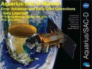
Aquarius/SAC-D Mission Error Validation and Early Orbit Corrections Gary Lagerloef 6 th Science Meeting; Seattle, WA, USA 19-21 July 2010. Three Phases. Pre-Launch In Orbit Checkout (Launch + 45 days) IOC + 6 months. Phase 1 – Pre-Launch.

E N D
Aquarius/SAC-D Mission Error Validation and Early Orbit Corrections Gary Lagerloef 6th Science Meeting; Seattle, WA, USA 19-21 July 2010
Three Phases • Pre-Launch • In Orbit Checkout (Launch + 45 days) • IOC + 6 months
Phase 1 – Pre-Launch • What: Generate a set of special case 7-day cycles • Specific cases: biases, drifts, etc, in following charts • How: Use the operational mission simulator. • Start with daily files from RSS • Add spurious signal for specific case study (see below) • Input these to the mission simulator as test cases. • Distribute and analyze (science team) • Timetable: • September: Produce a subset of scenarios (L2 files) • September-November: Analysis and assessment • December: Operational Readiness Review (ORR)
Scenario Flow Chart Daily simulated files (RSS & JPL) Apply spurious signals for special case studies Mission Simulator Telemetry files to/from Cordoba Generate special case telemetry files Level 1 > Level 2 > Level 3 Routine Processing Level 1 > Level 2 > Level 3 Special Case Processing Daily Mission Simulator L1, L2, L3 files uploaded to web site Special Case Simulator L1, L2, L3 files uploaded to evaluation products web site with documentation
Potential scenarios / rehearsals Simulate certain special situations to test and analyze Develop and test analysis tools Demonstrate we can address these issues at ORR • Insert arbitrary biases in all channels • Simulate arbitrary drifts in all channels • Orbit harmonics calibration drifts (1-4 harmonics, e.g.) • Simulate a complete cold sky maneuver • Solar flare • RFI • Attitude offsets & time tag offsets • Channel failure • H or V channel • P or M channel • Other suggestions … lunar, bi-static solar reflection, diffuse galaxy refl.
Arbitrary biases in all channels Generate test data: • Select a 7-day segment from the mission simulator input. • Add an arbitrary bias to each of the radiometer and scatterometer channels on each horn. • Process to L2 science data files, L3 bin-average and L3 smooth files. • Place the modified L1A, L2 and L3 files in an evaluation folder. Science Team Analysis: • Assess effects on L2 science data file TAs, U, Faraday, wind speed and SSS • Develop and evaluate bias detection/removal techniques, and assess uncertainties. • Inspect the impact on L3 files as a diagnostic tool. • Set up follow-on blind test with unknown biases.
Linear 7-day calibration drifts Generate test data: • Select a 7-day segment from the mission simulator input • Add arbitrary drift (~0.1K/ 7-days) to each of the radiometer and scatterometer channels on each horn. • Process to L2 science data files, L3 bin-average and L3 smooth files. • Set aside the modified L1A, L2 and L3 files in a special folder. Science Team Analysis: • Assess effects on L2 science data file TAs, U, Faraday, wind speed and SSS • Develop and evaluate drift detection/removal techniques, and assess uncertainties. • Inspect the impact on L3 files as a diagnostic tool. • Set up follow-on blind test with unknown drifts.
Harmonic orbital calibration drifts Generate test data: • Select a 7-day segment from the mission simulator input • Add arbitrary harmonic to each of the radiometer and scatterometer channels on each horn. (N cycles per orbit, N=1..3, with amplitudes ~0.1K) • Process to L2 science data files, L3 bin-average and L3 smooth files. • Set aside the modified L1A, L2 and L3 files in a special folder. Science Team Analysis: • Assess effects on L2 science data file TAs, U, Faraday, wind speed and SSS • Develop and evaluate drift detection/removal techniques, and assess uncertainties. • Inspect the impact on L3 files as a diagnostic tool. • Set up follow-on blind test with unknown drifts.
Phase 2 – In Orbit Checkout • Aquarius Commissioning phase timeline • Science Commissioning approach • Critical events and Science Tasks • Preliminary Acceptance Criteria
Aquarius Instrument Commissioning Timeline L+25 L+26 L+27 L+28 L+30 L+32 L+34 L+35 L+29 L+31 L+33 Time from launch (days) 11 days L+45 2 3 4 5 6 7 8 9 10 1 AQ Instrument Deployment & Checkout Phase Mission Phase SAC-D instruments on Upload patches AQ Activities Verify S/P config ICDS ON ICDS ATC On ATC Config ATC cntrlr Deply Boom Deply reflector Antenna Deployment Deply heaters on DPU off DPU On DPU + RFEs + RBEs ON DPU On Radiometer SCAT Rx only SCAT Tx single beam SCAT Tx ALL beam Scatterometer Instrument preliminary Performance assessment Post Launch Assessment Review PLAR Ground Coverage NEN Cordoba Matera Mission Design Team Product
Science Commissioning Approach • Post-launch in-orbit checkout simulation: During the period from launch to L+25 days, the science team will compute simulated Tb and σ0 based on the final orbit maneuvers (Science Task 1). • These data will provide “Expected Values” for each beam along-track to compare quantitatively with observations for both the engineering and science acceptance analyses. • The science team will carry out an analysis sequence (Science Tasks 2-7) at each stage of the instrument turn-on sequence. • Acceptance criteria are limited: • The timeline only allows for one 7-day cycle after the instrument is fully turned on. • Assess whether the data are “as expected” in qualitative terms and the sensor is “calibrate-able”. • Gross geographical and geophysical features are as expected, biases can be removed, stability is reasonable, polarization differences are appropriate, etc. (details below)
Preliminary Acceptance Criteria • Land versus ocean features are clearly evident, both in terms of brightness temperature (Tb) contrast and location. • V-H polarization differences for each incidence angle are consistent with the emissivity model • The 3rd Stokes is small. • Incidence angle effects such as the V-pol (H-pol) Tb increasing (decreasing) from the inner to outer beams consistent with emissivity model. • Relative stability is seen over known Earth targets such as Antarctic ice, rain forests, and ocean. • Scat σ0 sensitivity to wind speed within expectations for each channel • RFI detection and filtering are functional • No detectable scat-radiometer interference • No detectable radiometer interference from other SAC-D instruments • SSS biases will be removed via ground data matchups and crossover difference analysis; initial “first-look” 7-day map will be produced • We will also look for any large anomalous features that cannot be easily explained by expected calibration issues that usually occur early in a mission.
Phase 3 - IOC + 6 months Evaluate match-up data between Aquarius and in situ observing system • Provide preliminary SSS bias removal and un-validated science data • Monitor and analyze calibration drifts and biases • Asses systematic and geographically correlated errors • Analyze Scatterometer wind speed algorithm • Analyze roughness effects on TH, TV and salinity algorithm • And more….. Plan a science meeting for approximately IOC + 6 months • Asses calibration and validation results • Approve algorithm updates • Reprocess the first six months of data.
Approaches to De-biasing Search Radius Buoy Obs. • Each radiometer needs to be independently calibrated • First try to remove the gross offsets in the initial retrieved SSS • Use reference salinity field globally • AVDS matchups – tabulate for each beam • Cross-over analysis to remove residual inter-beam biases • With time, work through the re-calibration of retrieval coefficients • Match-up processing • One match-up file per buoy observation contains all the satellite data in the search radius • Subsequent processing to generate the optimal weighted average satellite observation per buoy • Global tabulations
Remove orbit errors and biases Cross over difference analysis to remove systematic errors between different beams Beam 1 SSS (with harmonic errors added) Beam 2 SSS (with constant and harmonic errors added) Adjusted Beam 1 SSS (with harmonic errors removed) Adjusted Beam 2 SSS (with constant and harmonic errors removed)
Validation Working Group • Review activities for these three phases • Pre-lauch • IOC • IOC + 6 months • Focus in ideas of the third phase
Validation - Theory The satellite salinity measurement SS and the in situ validation measurement SV are defined by: SS = S ± εS SV = S ± εV where S is the true surface salinity averaged over the Aquarius footprint area and microwave optical depth in sea water (~ 1 cm). εS and εV are the respective satellite and in situ measurement errors relative to S. The mean square of the difference ∆S between SS and SV is given by: <∆S2> = <εS2> + <εV2> where <> denotes the average over a given set of paired satellite and in situ measurements, and <εSεV> =0. Our objective is to validate that <εS2> = <∆S2>−<εV2> ≤ εR2 where εRis the allocated rms error requirement. The satellite measurement error is the difference between <∆S2> and mean square in situ error <εV2>.
Validation Errors εVis the rss of several terms: εPis thedifference error between a point salinity measurement and the area average over the instantaneous satellite footprint (log-normal distribution, median ~0.05 psu, extremes ~0.5). εOis an error due to the temporal or spatial offset between the satellite and in situ samples (many buoys surface once every 10 days and will be paired with the nearest satellite pass). εZis the difference error between the skin depth (~1-2 cm) salinity and in situ instrument measurement generally at 0.5 m to 5 m depth (can be >1 psu in rain). εCis the in situ sensor calibration error, usually very small (<0.05 psu)
εP =difference error between a point measurement and the area average Ship tracks spatially filtered and differenced with point measurements
εP =difference error between a point measurement and the area average Log normal εP ~ 0.05 psu
εO = error due to temporal or spatial offset between the satellite and in situ samples Distance from footprint center Nominally ~0.2 psu Spatial structure function from ship track data
εZ = difference error between the skin depth (~1-2 cm) salinity and in situ instrument 100 km TOGA/COARE R/V Wecoma Skin (2cm) vs 2m and 5m depths during heavy rain
Argo Enhanced SSS Float Trials Purpose: To obtain “skin” salinity and upper 5m gradient statistics • Argo CTD nominally shuts off at ~5m • Steve Riser and Gary Lagerloef are testing experimental Argo floats each with a secondary CTD sensor to profile to the surface. The primary CTD will shut off at ~5 m per normal operations. • Sea-Bird developed a specialized “Surface Temperature Salinity” (STS) sensor which is programmed to profile the upper ~30 m and is inter-calibrated with the primary CTD • We deployed the first at the HOT site near Hawaii late summer 2007. • 20 more have been funded by NASA and deployed in the past 2 years. (S.Riser) • New version funded including acoustic rain and wind measurements (S.Riser)
Validation Approach • Match co-located buoy and satellite observations globally. • Account for various surface measurement errors. • Sort match-ups by latitude (SST) zones. • Validate that the error allocations are met for the appropriate mean number of samples within the zone, or • Calculate global rms over monthly interval The Current Best Estimate (CBE) includes instrument errors plus all geophysical corrections such as surface roughness, atmosphere, rain, galaxy, solar, …