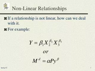
Non-continuous Relationships

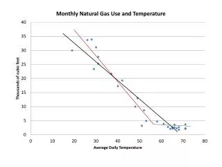
2. Non-continuous Relationships If the relationship between the dependent variable and an independent variable is non-continuous a slope dummy variable can be used to estimate two sets of coefficients and intercepts for the independent variable. For example, if natural gas usage is not affected by temperature when the temperature rises above 60 degrees, we could have: Gas usage = b0 + b1(GT60) + b2(Temp) + b3(GT60)(Temp) where GT60 is a dummy equal to 1 when the temperature is above 60 degrees

3. Non-continuous Relationships Note that at temperatures above 60 degrees the net effect of a 1 degree increase in temperature on gas usage is -0.056 (-.866+.810) and the estimated intercept is 6.4 (53.0-46.6)

4. Interaction Terms You can try to control for interactions between two variables by including a variable that is the product of two independent variables. For example, assume we were estimating the salaries of baseball players. If there was a premium paid to players that were both good fielders and good hitters, we might want to include an interaction term for hitting and fielding in the model.

5. Standardized Coefficients When the regression model is estimated after standardizing the values of the dependent and independent variables.

6. Standardized Coefficients Standardized coefficients can be used to compare the magnitude of the effects of the independent variables. Unstandardized Standardized Coefficients Coefficients B Std.Err. Beta t Sig. (Constant) -14.485 4.038 -3.587 .000 Weight -.007 .000 -.706 -14.177 .000 Year .761 .050 .360 15.262 .000 Cylinders -.074 .232 -.016 -.320 .749 a Dependent Variable: MPG

7. Standardized Residuals Where s is the standard error of estimate and hi is the leverage of observation i. Leverage is determined by the difference between the value of the independent variables and their means.

8. Standardized Residuals The random deviation in the value of y, e, is assumed to be normally distributed. Looking at the standardized residuals gives some indication if that is true. Values should lie within 2 standard deviations of 0. Values greater than 2 may indicate the presence of outliers.

9. Residuals for MPG Example

10. Distribution of Standardized Residuals

11. Summary of Issues in Building Models • Check for multicollinearity • Look for outliers • Check residuals for nonlinear relationships • Check residuals for hetroscedasticy • Were all relevant variables included?

12. Time Series Data Observations on a variable measured over successive periods of time.

13. Components of a Time Series Trend – The long-run movement of a time series Seasonal component – The component of a time series that shows a periodic pattern over a year Cyclical component – The component of a time series related to the business cycle Irregular component – The random variation in a time series not accounted for by the other components

14. Smoothing a Time Series Smoothing removes the irregular component of a time series. It can be used to forecast if the variable has no significant trend, cyclical, or seasonal effects. It can also be used to investigate whether there is a trend in the data.

15. Smoothing Techniques Moving average: Weighted moving average: A moving average in which more recent values are given heavier weights Exponential smoothing: When the weight on an observation decreases exponentially as time passes

16. Example, Moving Averages Where the weights are .1, .2, .3, and .4; oldest to most recent

17. Exponential Smoothing Ft+1 = aYt + (1 – a)Ft Ft+1 = Forecast for period t+1 a = Smoothing constant Yt = Value of the time series in period t Ft = Forecast for time t

18. Example, Moving Averages Assumes a equals 0.6

19. Estimating the Trend Tt = b0 + b1t Tt = trend value of time series in period t b0 = intercept in trend line b1 = slope of trend line t = time

20. Example, Trend Tt = 104 + 10.5(t)

21. Time Series and Trend

22. Time Series and Nonlinear Trends

23. Nonlinear Trends • Make the trend a nonlinear function of time, such as: • y = b0 + b1t + b2t2 • If there is a constant percentage change in y over time use the natural log of y as the dependent variable: • ln(y) = b0 + b1t • Which corresponds to: • y = b0(tb1)

24. Cyclical Variation If there is cyclical variation there will be evidence of a correlation between the variable and GDP (remember to adjust for inflation). When forecasting you would need to include a leading indicator into the model. Yt = b0 + b1t +b2(housing starts in t-1)

25. Seasonal Variation Seasonal index – Assumes there is a constant percentage difference from the trend in a given season

26. Seasonal Index Interpret the index as the ratio of the average value for that season to the average for the year. How would you interpret an index value of 0.9 for the first quarter? On average values in the first quarter are 90% of the annual average. What if the index for the 2nd quarter was 1.20? On average values in the 2nd quarter are 20% above the annual average

28. Examples Assume the following quarterly indices: Q1 0.8 Q2 1.1 Q3 0.7 Q4 1.4 Deseasonalize the following data: Q1 Q2 Q3 Q4 400 660 560 700 500 600 800 500

29. Examples Assume t equals 1 in the first quarter of 2002 and the estimated trend for sales is T = 100 + 50t. What is the forecast for the 4th quarter of 2009? T = 100 + 50(32) = 1700 What is the seasonalized forecast? 1700(1.4) = 2380