Download
1 / 41
410 likes | 502 Views
Chapter 3 outlines how to describe numerical and graphical summaries, simple and multiple linear regression models, and diagnostic tools for analyzing relationships in data. Learn to interpret scatterplots, correlation, statistical models, and regression results effectively. Understand assumptions and how to check for violations.

E N D
Outline • Describing: Numerical summaries Graphical summaries • Simple linear regression: Model Inferences Diagnostics • Multiple linear regression: Linear regression ANCOVA
Scatterplots • Plot two-variable relationships. • A point represents a value for each variable. • Points can be described: Direction (positive or negative) Linear Strength
Scatterplots Insert Figure 3-1
Correlation Correlation ranges between 1 and 1. 1—strongest negative linear relationship +1—strongest positive linear relationship 0—no linear relationship
Correlation *p-Value < 0.05.
What is a Linear Relationship? Insert Figure 3-4
Statistical Models • Help us understand relationships in the data and how the data could have been produced. • Relate a response to an explanatory variable. • Define how changes in the response variable can be explained by the explanatory variable. • Provide a mechanism for understanding the random variation that may occur in the relationship between the response and the explanatory variables.
Statistical Model The scatter plots indicate that there might be a linear relationship between tap water consumption and hemoglobin change. This suggests that a line would do a good job of describing the relationship.
Random Variation Insert Figure 3-5 We would not expect data to line up perfectly.
Simple Linear Regression Model Response = + (explanatory variable) + • Identically and Independently distributed as normals • Mean of 0 • Constant variance
Least Squares Insert Figure 3-7 How do you choose the line? Minimize the errors.
Explaining Variability Insert Figure 3-8 R2 is the proportion of variability explained by the regression model (x).
Prediction Equation The prediction equation is the estimated line. Can be used to predict responses, Note: No error term – this is not a “model;” this is an actual line.
Diagnostics • Linear regression assumptions: The mean of the errors is 0. The errors have constant variance. The errors are identically and independently distributed as normals. • Checking the assumptions: Plots Residuals Outliers and influence points
Residual Plots • The plot of the residuals vseach of the regressorvariables: Should be random . Scattergramsshould occur at the horizontal line 0. • Nonrandom scatter on residual plots indicates violations of model assumptions.
Residual Plots: Potential violations • Studentized residuals vs predicted can indicate an outlier. • Studentized residuals vs predicted can indicate nonconstantvariance (V-shaped plot). • Studentized residuals vsgiven predictor can indicate need for higher order terms (curvilinear plot). • Studentized residuals vs time can indicate correlation among residuals (sine curve plot). (really not an issue with cross-sectional data)
Insert Figure 3-12 Residual vsx: If all assumptions are met, your plot might look like this.
Insert Figure 3-13 A violation has occurred...how can you tell?
Insert Figure 3-14c A violation has occurred...how can you tell?
Insert Figure 3-18b A violation has occurred...how can you tell?
Polynomial Regression • When a curve is leftover in the residuals, you might need to add a polynomial term. For example, remember the formula for a parabola quadratic regression (includes a squared term): Usually happens with variables like age
Statistical Models You are already familiar with a statistical model that describes the linear relationship between X and Y. Y = + X+ ε, εN(0,2) Simple linear regression
Multiple Linear Regression • Public health involves complex research problems; so, it is not often that there is only one explanatory variable or one regressor (x). • When there are multiple regressors, we have multiple linear regression: y = + 1x1 + 2x2 + … + KxK + • For the purposes of illustration, let us start with two regressors x1 and x2.
Two-Regressor Model • The model: yi= α +1x1i + 2x2i + i, i= 1,..., n • Model assumptions: 1, 2,…, n represents a random sample of unobservable error terms from a population of residuals characterized by • Mean (i) = 0 for all the i’s • Var (i) = 2 for all the i’s(homoscedasticity) • Cov (i, j) = 0 for all the i’s ≠ j’s(another way of saying independent)
Obtaining Estimates (Two Regressors) • To obtain estimates for , 1, 2, and 2, use the same principle of least squares as you did in simple linear regression. Minimize the SSE!
More than Two Regressors Essentially the same as with two regressors, just more variables in the model y = + 1x1 + 2x2 + … + kxk + Additional issue: The regressors cannot be highly correlated.
Collinearity • If correlation between two regressorsis near +1 or 1, we say that the regressors are collinear. b1 and b2, the least squares estimates of 1 and 2 are • often large in value, • approximately equal, but • have opposite signs The SE of the estimates are also large, implying that the t-tests for testing H0: 1=0 and H0: 2=0 are not significant.
Problems with Collinearity(Two Regressors) • When there is collinearity The overall F-test in the ANOVA table is statistically significant (at least one of the ’s and possibly both are not zero) . The t-tests do not clarify which is not zero.
Confounding • A confounding variable is a variable that is associated with both the disease and the exposure variable. • Confounding occurs when an estimate is distorted by the effect of variables that are also risk factors for the outcome. • A confounder is associated with BOTH the exposure and the outcome of interest.
X Y X Y F Confounding • Suppose you are studying whether x is a cause of y. • F is a confounder if the following is true.
When is it reasonable to control for confounding? • Depends on whether or not the confounder is in the causal pathway between “exposure” and “disease.” “Exposure” is causally related to the confounder. The confounder is causally related to the “disease.”
Controlling Confounding • In the design stage, you can Restrict (inclusion criterion controls for confounding) Match • In the analysis stage, you can Do a stratified analysis (or standardization) Perform mathematical modeling • Regression techniques (e.g., ANCOVA) • Propensity scores
Variable Selection • Depends somewhat on the purpose of the regression analysis. Prediction/Forecasting Covariate-adjustment • Be careful about automated techniques.