Download
1 / 26
260 likes | 419 Views
Issues in factorial design. No main effects but interaction present. Can I have a significant interaction without significant main effects? Yes Consider the following table of means. No main effects but interaction present.

E N D
No main effects but interaction present • Can I have a significant interaction without significant main effects? • Yes • Consider the following table of means
No main effects but interaction present • We can see from the marginal means that there is no difference in the levels of A, nor difference in the levels of factor B • However, look at the graphical display
No main effects but interaction present • In such a scenario we may have a significant interaction without any significant main effects • Again, the interaction is testing for differences among cell means after factoring out the main effects • Interpret the interaction as normal
Robustitude • As in most statistical situations there would be a more robust method for going about factorial anova • Instead of using means, we might prefer trimmed means or medians so as to have tests based on estimates not so heavily influenced by outliers. • And, there’s nothing to it.
Between subjects factorial using trimmed means Interaction Main effects
Robustitude • Or using R you type in something along the lines of • t2way(A, B, x, grp=c(1:p), tr=.2, alpha=.05) • Again, don’t be afraid to try robust methods as they are often easily implemented with appropriate software.
Unequal sample sizes • Along with the typical assumptions of Anova, we are in effect assuming equal cell sizes as well • In non-experimental situations, there will be unequal numbers of observations in each cell • Semester/time period for collection ends and you need to graduate • Quasi-experimental design • Participants fail to arrive for testing • Data are lost etc. • In factorial designs, the solution to this problem is not simple • Factor and interaction effects are not independent • Do not total up to SSb/t • Interpretation can be seriously compromised • No general, agreed upon solution
Non-drinking Drinking Row means Michigan Arizona Column means The problem (Howell example) • Drinking participants made on average 6 more errors, regardless of whether they came from Michigan or Arizona • No differences between Michigan and Arizona participants in that regard
Example • However, there is a difference in the row means as if there were a difference between States • Occurs because there are unequal number of participants in the cells • In general, we do not wish sample sizes to influence how we interpret differences between means • What can be done?
Another example • How men and women differ in their reports of depression on the HADS (Hospital Anxiety and Depression Scale), and whether this difference depends on ethnicity. • 2 independent variables--Gender (Male/Female) and Ethnicity (White/Black/Other), and one dependent variable-- HADS score.
Note the difference in gender • 2.47 vs. 4.73 • A simple t-test would show this difference to be statistically significant and noticeable effect
Unequal sample sizes • Note that when the factorial anova is conducted, the gender difference disappears • It’s reflecting that there is no difference by simply using the cell means to calculate the means for each gender • (1.48+6.6+12.56)/3 vs. (2.71+6.26+11.93)/3
Unequal sample sizes • What do we do? • One common method is the unweighted (i.e. equally weighted)-means solution • Average means without weighting them by the number of observations • Note that in such situations SStotal is usually not shown in ANOVA tables as the separate sums of squares do not usually sum to SStotal
Unequal sample sizes • In the drinking example, the unweighted means solution gives the desired result • Use the harmonic mean of our sample sizes • No state difference • 17 v 17 • With the HADS data this was actually part of the problem • The t-test would be using the weighted means, the anova the ‘unweighted’ means • However, with the HADS data the tests of simple effects would bear out the gender difference and as these would be part of the analysis, such a result would not be missed • In fact the gender difference is largely only for the white category • i.e. there really was no main effect of gender in the anova design
A note about proportionality • Unequal cells are not always a problem • Consider the following tables of sample sizes
The cell sizes in the first table are proportional b/c their relative values are constant across all rows (1:2:4) and columns (1:2) • Table 2 is not proportional • Row 1 (1:4:2) • Row 2 (1:1:5)
Proportionality • Equal cells are a special case of proportional cell sizes • As such, as long as we have proportional cell sizes we are ok with traditional analysis • With nonproportional cell sizes, the factors become correlated and the greater the departure from proportional, the more overlap of main effects
More complex design: the 3-way interaction • Before we had the levels of one variable changing over the levels of another • So what’s going on with a 3-way interaction? • How would a 3-way interaction be interpreted?
2 X 2 X 2 Example *Sometimes you will see interactions referred to as ordinal or disordinal, with the latter we have a reversal of treatment effect within the range of some factor being considered (as in the left graph).
Interpretation • An interaction between 2 variables is changing over the levels of another (third) variable • Interaction is interacting with another variable • AB interaction depends on C • Recall that our main effects would have their interpretation limited by a significant interaction • Main effects interpretation is not exactly clear without an understanding of the interaction • In other words, because of the significant interaction, the main effect we see for a factor would not be the same over the levels of another • In a similar manner, our 2-way interactions’ interpretation would be limited by a significant 3-way interaction
Simple effects • Same for the 2-way interactions • However now we have simple, simple main effects (differences in the levels of A at each BC) and simple interaction effects
Simple effects • In this 3 X 3 X 2 example, the simple interaction of BC is nonsignificant, and that does not change over the levels of A (nonsig ABC interaction) • Consider these other situations
Simple effects • As mentioned previously, a nonsignificant interaction does not necessarily mean that the simple effects are not significant as simple effects are not just a breakdown of the interaction but the interaction plus main effect • In a 3-way design, one can test for simple interaction effects in the presence of a nonsignificant 3-way interaction • The issue now arises that in testing simple, simple effects, one would have at minimum four comparisons (for a 2X2X2), • Some examples are provided on the website using both the GLM and MANOVA procedures. Here is another from our backyard: • http://www.coe.unt.edu/brookshire/spss3way.htm#simpsimp