Download

1 / 84
920 likes | 1.38k Views
IE440:PROCESS IMPROVEMENT THROUGH PLANNED EXPERIMENTATION. The 2 K Factorial Design. Dr. Xueping Li Dept. of Industrial & Information Engineering University of Tennessee, Knoxville. Design of Engineering Experiments Part 4 – Introduction to Factorials. Text reference, Chapter 6

E N D
IE440:PROCESS IMPROVEMENT THROUGH PLANNED EXPERIMENTATION The 2K Factorial Design Dr. Xueping Li Dept. of Industrial & Information Engineering University of Tennessee, Knoxville
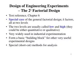
Design of Engineering ExperimentsPart 4 – Introduction to Factorials • Text reference, Chapter 6 • The 22 Design • The 23 Design • The general 2K Design • The addition of center points to the 2K design
Chemical Process Example A = reactant concentration, B = catalyst amount, y = recovery
The Simplest Case: The 22 “-” and “+” denote the low and high levels of a factor, respectively Low and high are arbitrary terms Geometrically, the four runs form the corners of a square Factors can be quantitative or qualitative, although their treatment in the final model will be different
22 Factorial Design Involves two factors (A and B) and n replicates. We are interested in: • main effect of A, • main effect of B, and • interaction between A and B.
Estimation of Factor Effects See textbook, pg. 205-206 For manual calculations The effect estimates are: A = 8.33, B = -5.00, AB = 1.67 Practical interpretation? Design-Expertanalysis
Table 6.2 (p. 208)Algebraic Signs for Calculating Effects in the 22 Design Standard order/Yate’s order
Figure 6.1 (p. 204)Treatment combinations in the 22 design. Contrast ::=combinations (*) signs Effects ::=2constrast/[n*2^(k)] SS ::=constrast^2/[n*2^(k)]
Table 6.1 (p. 208)Analysis of Variance for the Experiment in Figure 6.1
The Regression Model • The regression model • Coded variable vs. natural variable • X_Coded= [Var – (Var_L+Var_H)/2 ]/(Var_H – Var_L)/2 • Var = X_Coded * (Var_H – Var_L)/2 + (Var_L+Var_H)/2
Figure 6.2 (p. 210)Residual plots for the chemical process experiment.
Figure 6.3 (p. 211)Response surface plot and contour plot of yield from the chemical process experiment.
The 23 factorial design. Figure 6.4 (p. 211)The 23 factorial design.
Figure 6.5 (p. 213)Geometric presentation of contrasts corresponding to the main effects and interactions in the 23 design.
Table 6.3 (p. 214)Algebraic Signs for Calculating Effects in the 23 Design
Figure 6.6 (p. 216)The 23 design for the plasma etch experiment for Example 6-1.
Table 6.6 (p. 218)Analysis of Variance for the Plasma Etching Experiment
Figure 6.7 (p. 219)Response surface and contour plot of etch rate for Example 6-1.
To-do-list • Project
Figure 6.9 (p. 227)The impact of the choice of factor levels in an unreplicated design.
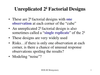
Unreplicated 2kFactorial Designs • Lack of replication causes potential problems in statistical testing • Replication admits an estimate of “pure error” (a better phrase is an internal estimate of error) • With no replication, fitting the full model results in zero degrees of freedom for error • Potential solutions to this problem • Pooling high-order interactions to estimate error • Normal probability plotting of effects (Daniels, 1959) • Other methods…see text, pp. 234
Example of an Unreplicated 2k Design • A 24 factorial was used to investigate the effects of four factors on the filtration rate of a resin • The factors are A = temperature, B = pressure, C = mole ratio, D= stirring rate • Experiment was performed in a pilot plant
Figure 6.10 (p. 228)Data from the pilot plant filtration rate experiment for Example 6-2.
Table 6.12 (p. 229)Factor Effect Estimates and Sums of Squares for the 24 Factorial in Example 6.2
Figure 6.11 (p. 230)Normal probability plot of the effects for the 24 factorial in Example 6-2.
Figure 6.12 (p. 230)Main effect and interaction plots for Example 6-2.
Table 6.13 (p. 231)Analysis of Variance for the Pilot Plant Filtration Rate Experiment in A, C, and D.
Figure 6.13 (p. 233)Normal probability plot of residuals for Example 6-2.
Figure 6.14 (p. 233)Contour plots of filtration rate, Example 6-2.
Figure 6.15 (p. 234)Half-normal plot of the factor effects from Example 6-2.
Figure 6.17 (p. 237)Data from the drilling experiment of Example 6-3.
Figure 6.18 (p. 237)Normal probability plot of effects for Example 6-3.
Figure 6.19 (p. 237)Normal probability plot of residuals for Example 6-3.
Figure 6.20 (p. 237)Plot of residuals versus predicted rate for Example 6-3.