Download
1 / 15
180 likes | 508 Views
Chapter 5. Discrete-Time Process Models. Discrete-Time Transfer Functions. Now let us calculate the transient response of a combined discrete-time and continuous-time system, as shown below. The input to the continuous-time system G ( s ) is the signal:.

E N D
Chapter 5 Discrete-Time Process Models Discrete-Time Transfer Functions • Now let us calculate the transient response of a combined discrete-time and continuous-time system, as shown below. • The input to the continuous-time system G(s) is the signal: • The system response is given by the convolution integral:
Chapter 5 Discrete-Time Process Models Discrete-Time Transfer Functions • With • For 0 ≤ τ ≤ t, • We assume that the output sampler is ideally synchronized with the input sampler. • The output sampler gives the signal y*(t) whose values are the same as y(t) in every sampling instant t = jTs. • Applying the Z-transform yields:
Chapter 5 Discrete-Time Process Models Discrete-Time Transfer Functions • Taking i = j – k, then: • For zero initial conditions, g(iTs) = 0, i < 0, thus: where • Discrete-time Transfer Function • The Z-transform of Continuous-time Transfer Function G(s) • The Z-transform of Input Signal u(t)
Chapter 5 Discrete-Time Process Models Discrete-Time Transfer Functions • When the sample-and-hold device is assumed to be a zero-order hold, then the relation between G(s) and G(z) is
Chapter 5 Discrete-Time Process Models Example Find the discrete-time transfer function of a continuous system given by: where
Chapter 5 Discrete-Time Process Models Approximation of Z-Transform • Previous example shows how the Z-transform of a function written in s-Domain can be so complicated and tedious. • Now, several methods that can be used to approximate the Z-transform will be presented. • Consider the integrator block as shown below: • The integration result for one sampling period of Ts is:
Chapter 5 Discrete-Time Process Models Approximation of Z-Transform • Forward Difference Approximation (Euler Approximation) The exact integration operation presented before will now be approximated using Forward Difference Approximation. • This method follows the equation given as: • Taking the Z-transform of the above equation: while • Thus, the Forward Difference Approximation is done by taking or
Chapter 5 Discrete-Time Process Models Approximation of Z-Transform • Backward Difference Approximation The exact integration operation will now be approximated using Backward Difference Approximation. • This method follows the equation given as: • Taking the Z-transform of the above equation: while • Thus, the Forward Difference Approximation is done by taking or
Chapter 5 Discrete-Time Process Models Approximation of Z-Transform • Trapezoidal Approximation(Tustin Approximation, Bilinear Approximation) The exact integration operation will now be approximated using Backward Difference Approximation. • This method follows the equation given as: • Taking the Z-transform, while • Thus, the Forward Difference Approximation is done by taking or
Chapter 5 Discrete-Time Process Models Example Find the discrete-time transfer function of for the sampling time of Ts = 0.5 s, by using (a) ZOH, (b) FDA, (c) BDA, (d) TA. (a) ZOH (b) FDA
Chapter 5 Discrete-Time Process Models Example (c) BDA (d) TA
Chapter 5 Discrete-Time Process Models Input-Output Discrete-Time Models • A general discrete-time linear model can be written in time domain as: where m and n are the order of numerator and denominator, k denotes the time instant, and d is the time delay. • Defining a shift operator q–1, where: • Then, the first equation can be rewritten as: or or
Chapter 5 Discrete-Time Process Models Input-Output Discrete-Time Models • The polynomials A(q–1) and B(q–1) are in descending order q–1, completely written as follows:
Chapter 5 Discrete-Time Process Models Homework 6 (a) Find the discrete-time transfer functions of the following continuous-time transfer function, for Ts = 0.25 s and Ts = 1 s. Use the Forward Difference Approximation (b) Calculate the step response of both transfer functions for 0 ≤ t ≤ 5 s. (c) Compare the step response of both transfer functions with the step response of the continuous-time transfer function G(s) in one plot.