Chapter 10 Stability Analysis and Controller Tuning
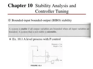
Chapter 10 Stability Analysis and Controller Tuning. ※ Bounded-input bounded-output (BIBO) stability. * Ex. 10.1 A level process with P control. (S1) Models (S2) Solution by Laplace transform. where. Note: Stable if K c <0 Unstable K c >0 Steady state performance by.

Chapter 10 Stability Analysis and Controller Tuning
E N D
Presentation Transcript
Chapter 10 Stability Analysis and Controller Tuning ※ Bounded-input bounded-output (BIBO) stability * Ex. 10.1 A level process with P control
(S1) Models (S2) Solution by Laplace transform where
Note: • Stable if Kc<0 • Unstable Kc>0 • Steady state performance by
* Ex. 10.3 A level process without control • Response to a sine flow disturbance • Response to a step flow disturbance
* Stability of linearized closed-loop systems Ex. 10.4 The series chemical reactors with PI controller
@ Known values • Process • Controller
@ Formulation& stability Stable
◎ Criterion of stability ※ Direct substitution method
﹪Ultimate gain (Kcu): The controller gain at which this point of marginal instability is reached ﹪Ultimate period (Tu): It shows the period of the oscillation at the ultimate gain * Using the direct substitution method by in the characteristic equation
Find: (1) Ultimate gain (2) Ultimate period S1. Characteristic eqn.
Example A.2 S1.
S2. S3.
Example A.3 Find the following control loop: (1) Ultimate gain (2) Ultimate period
S1. The characteristic eqn. for H(s)=KT/(Ts+1) S2. Gc=-Kc to avoid the negative gains in the characteristic eqn.
* Dead-time Since the direct substitution method fails when any of blocks on the loop contains deadt-ime term, an approximation to the dead-time transfer function is used. First-order Padé approximation:
Example A.4 Find the ultimate gain and frequency of first-order plus dead-time process S1. Closed-loop system with P control
Note: • The ultimate gain goes to infinite as the dead-time approach zero. • The ultimate frequency increases as the dead time decreases.
※ Root locus A graphical technique consists of roots of characteristic equation and control loop parameter changes.
*Definition: Characteristic equation: Open-loop transfer function (OLTF): Generalized OLTF:
Example B.1: a characteristic equation is given S1. Decide open-loop poles and zeros by OLTF
S2. Depict by the polynomial (characteristic equation) Kc:1/3
Example B.2: a characteristic equation is given S1. Decide poles and zeros
Example B.3: a characteristic equation is given S1. Decide poles and zeros S2. Depict by the polynomial (characteristic equation)
@ Review of complex number c=a+ib
P1. Multiplication for two complex numbers (c, p) P2. Division for two complex numbers (c, p)
@ Rules for root locus diagram • Characteristic equation • Magnitude and angle conditions
Rule for searching roots of characteristic equation • Ex. A system have two OLTF poles (x) and one OLTF zero (o) • Note: If the angle condition is satisfied, then the point s1 is the part of the root locus
Example B.4 Depict the root locus of a characteristic equation (heat exchanger control loop with P control) S1. OLTF
S2. Rule for root locus • From rule 1 where the root locus exists are indicated. • From rule 2 indicate that the root locus is originated at the poles of OLTF. • n=3, three branches or loci are indicated. • Because m=0 (zeros), all loci approach infinity as Kc increases. • Determine CG=-0.155 and asymptotes with angles, =60°, 180 °, 300 °. • Calculate the breakaway point by
s= – 0.247 and –0.063 S3. Depict the possible root locus with ωu=0.22 (direct substitution method) and Kcu=24