Download
1 / 52
530 likes | 859 Views
Non-local means: a look at non-local self-similarity of images. IT 530, LECTURE NOTES. Partial Differential Equations (PDEs): Heat Equation. Executing several iterations of this PDE on a noisy image is equivalent to convolving the same image with a Gaussian!

E N D
Non-local means: a look at non-local self-similarity of images IT 530, LECTURE NOTES
Partial Differential Equations (PDEs): Heat Equation Executing several iterations of this PDE on a noisy image is equivalent to convolving the same image with a Gaussian! The “sigma” of the Gaussian is directly proportional to the number of time-steps of the PDE. • Inspired from thermodynamics • Blurs out edges
PDEs: Anisotropic Diffusion • Diffusivity function “g”. • Decreasing function of gradient magnitude. • Preserve edges: Diffuse along edges not across. Several papers: Perona and Malik [IEEE PAMI 1990], Total variation method [Rudinet al, 1992], Beltrami flow [Sochenet al, IEEE TIP 1998], etc.
PDEs: Total Variation • Total variation denoising seeks to minimize the following energy functional: Euler-Lagrange equation (Partial differential equation): exhibits anisotropic behaviour due to gradient magnitude term in the denominator. Diffusion is low across strong edges.
Heat equation Perona-Malik PDE Total variation
Neighborhood Filters for Denoising Simple averaging filter – will cause blurring of edges and textures in the image
Neighborhood Filters for Denoising: Lee Filter • Weigh the pixels in the neighborhood by factors inversely proportional to the distance between the central pixel and the particular pixel used for weighting. • This is expressed as: More weight to nearby pixels
Anisotropic Neighborhood Filter (Yaroslavsky Filter) • Weigh the pixels in the neighborhood by factors inversely proportional to the difference between the intensity values at those pixels and the intensity value of the pixel to be denoised. • This is expressed as: More weight to pixels with similar intensity values: better preservation of edges/boundaries
Bilateral Filter (Lee+Yaroslavsky Filter) • Weigh the pixels in the neighborhood by factors inversely proportional to the difference between the intensity values at those pixels and the intensity value of the pixel to be denoised, and the difference in pixel locations. • This is expressed as: More weight to pixels with similar intensity values: better preservation of edges/boundaries
Comparative Results • The anisotropic diffusion algorithm performs better than the others. • In the Yaroslavsky/Bilateral filter, the comparison between the intensity values is not very robust. This creates artifacts around the edges. • Performance difference between Yaroslavsky and bilateral filter is minor. • All aforementioned filter are based on the principle of piece-wise constant intensity images.
Non-local self-similarity Non-local self-similarity is very useful in denoising (and almost everything else in image processing). For denoising, you could simply take an average of all those patches that were “similar” (modulo noise).
Non-local Means Natural images have a great deal of redundancy: patches from different regions can be very similar NL-Means: a non-local pixel-based method (Buadeset al, 2005) • Awate and Whitaker (PAMI 2007) • Popat and Picard (TIP 1998) • De-Bonet (MIT Tech report 1998) • Wang et al (IEEE SPL 2003) Difference between patches
Non-local means: Basic Principle • Non-local means compares entire patches (not individual pixel intensity values) to compute weights for denoising pixel intensities. • Comparison of entire patches is more robust, i.e. if two patches are similar in a noisy image, they will be similar in the underlying clean image with very high probability. • We will see this informally and prove it mathematically in due course.
Non-local means: Variant Euclidean distance between two patches is being weighted by a Gaussian with maximum weight at the center of the two patches and decaying outwards
Three principles to evaluate denoising algorithms • (1): The residual image (also called “method noise”) – defined as the difference between the noisy image and the denoised image – should look like (and have all the properties of) a pure noise image. • (2): A denoising algorithm should transform a pure noise image into another noise image (of lower variance). • (3): A competent denoising algorithm should find for any pixel ‘i’, all and only those pixels ‘j’ that have the same model as ‘i’ (i.e. those pixels whose intensity would have most likely been the same as that of ‘i’, if there were no noise).
Principle 3: Correct models? The pixels with high weight in anisotropic diffusion or bilateral filters do NOT line up with our expectation (in all images!). This is because noise affects the gradient computation or single intensity driven weights. In NL-means, the comparison between patches is MUCH more robust to noise!
Non-local means: Implementation details • A drawback of the algorithm is its very high time complexity – O(N x N) for an image with N pixels. • Heuristic work-around: given a reference patch, restrict the research for similar patches to a window of size S x S (called as “search zone”) around the center of the reference patch.
Non-local means implementation details • The parameter sigma to compute the weights will depend on the noise variance. Heuristic relation is: • Patch-size is a free parameter – usually some size between 7 x 7 and 21 x 21 is chosen. Larger patch-size – better discrimination of the truly similar patches, but more expensive and more (over)smoothing. • Smaller patch-size – less smoothing.
Patch-size selection Patch-size too small: mottling effect (fake edges/patterns in constant intensity regions) Patch-size too large: oversmoothing of subtle textures and edges Ref: Duval and Gousseau, “A bias-variance approach for the non-local means”
Gray region (containing patch P) Ref: Duval and Gousseau, “A bias-variance approach for the non-local means” Black region (containing patch Q) Noisy gray region (containing patch U(x))
Assume patch-size is s x s. Assume noise from N(0,1). This is a zero-mean Gaussian random variable with variance 1 Discriminability improves as patch-size increases! It explains why NL-means outperforms single-pixel neighborhood filters! By definition of erfc, this probability decreases as ‘s’ increases.
Extension to Video denoising • For video-denoising, simply denoising each individual frame independently ignores temporal similarity or redundancy. • Most video denoising algorithms first perform a motion compensation step: (1) estimate the motion between consecutive frames, and (2) align each successive frame to its previous frame. • Motion estimation is performed typically by exploiting the “brightness constancy assumption”, i.e. that the intensity of any physical point is unchanged throughout the video.
Extension to Video denoising • The most popular motion compensation algorithms also assume that the motion of nearby pixels is similar (motion smoothness assumption). • You will study this in more detail in computer vision: optical flow. • Denoising is done after motion compensation (assuming that pixels at the same coordinate in successive frames will have same/similar intensities).
Extension to Video denoising • There are some problems in motion estimation, even more so, if the video is noisy. • One such issue is called the aperture problem – for any block in one frame, there are many matching blocks in the next frame.
Extension to video denoising • The motion smoothness assumption is one way to alleviate the aperture problem (again, you will study this in more detail in computer vision). • On the next slide, we will see the performance of the Lee filter and the Yaroslavsky filter, with and without motion compensation.
NL-Means for video denoising • Video data has tremendous redundancy (more than individual frames). • Any reference patch in one frame will have many similar patches in other frames – the aperture problem is NO problem for video denoising! • So forget about motion compensation! • Run NL-means on each frame, using similar patches from that frame as well as from nearby frames. • Advantages: avoids all the inevitable errors in motion estimation, AND saves computational cost!
An information-theoretic (and iterated) variant of NL-Means - UINTA • UINTA = Unsupervised information-theoretic adaptive filter. • UINTA is again based on the principle of non-local similarity. • It uses tools from information theory (conditional entropy) and kernel density estimation. • Uses a simple observation about the entropy of natural images. Ref: Awate and Whitaker, Higher-order image statistics for unsupervised, information-theoretic, adaptive image filtering”
Principle of UINTA • The conditional entropy of the intensity of a central pixel given its neighbors is low in a “clean” natural image. • As noise is added, this entropy increases. y1 y2 y5 To denoise, you can minimize the following quantity at each pixel: X y20 y24
Overview of UINTA algorithm • For each pixel location i, we seek to minimize the following quantity: • For this do a gradient descent (at each location) until convergence:
Mathematical details • For image neighborhoods with n pixels, we first need to estimate probability density functions of random variables having n (or n-1) dimensions. • Consider the neighborhoods are denoted as follows: • The expression for the PDF of Z is as follows:
Mathematical Details • The expression for the entropy is: • The gradient descent is given on the following slide.
Central pixel to be denoised Neighborhood Independent of value of x Chain rule A projection vector that extracts only the dimension corresponding to the central pixel
Note! Note! If you set the derivative of the conditional entropy to zero (you do this since you want to minimize the conditional entropy) and rearrange the terms, you get the NL-means update for denoising. So UINTA can be considered an iterated form of NL-means!
Earlier work on non-local similarity • A technique similar (in principle) to UINTA was developed by Popat and Picard in 1997. • A training set of clean and degraded images was used to learn the joint probability density of degraded neighborhoods and clean central pixels. • Given a noisy image, a pixel value is restored using an MAP estimate. • Unlike UINTA, this method requires prior training.
Texture synthesis or completion: another use of non-local similarity Ref: Efros and Leung, “Texture Synthesis by Non-parametric sampling” Remember: a texture image contains very high repetition of “similar” patches all over!
Method: • For every pixel (x,y) that needs to be filled, collect valid neighboring intensity values. • Search throughout the image to find “similar” neighborhoods. • Assign the intensity at (x,y) as some weighted combination of such central pixel values. • Free parameters: size of the neighborhood and the definition of “similar neighborhoods”. • For pseudo-code, see http://graphics.cs.cmu.edu/people/efros/research/EfrosLeung.html