Feature Similarity
Feature Similarity. 02/11/2002 Hyung Wook Park. The table of contents. Introduction. From Images to Similarity. From Features to Similarity. Similarity Between Two Sets of Points. Introduction. In the field of image retrieval - needed achieving a compact representation of .

Feature Similarity
E N D
Presentation Transcript
Feature Similarity 02/11/2002 Hyung Wook Park
The table of contents • Introduction • From Images to Similarity • From Features to Similarity • Similarity Between Two Sets of Points
Introduction • In the field of image retrieval - needed achieving a compact representation of image content using concise but effective feature • Their effectiveness depends on the fact that the notion of similarity between two images is subjective • Pre-attentive search techniques emphasize the need of descriptions of images and similarity measures or metrics to compare these description
Pre-attentive vs. Attentive Similarities • Pre-attentive similarity Determines the similarity of the stimuli without attempting their interpretation • Attentive similarity Determines the similarity between two stimuli after they have been interpreted and classified
Pre-attentive vs. Attentive Similarities It looks like quite similar
Pre-attentive vs. Attentive Similarities The difference between the two should be striking now
Pre-attentive vs. Attentive Similarities • Let Q : the query proposed by user U I : an image of the database Using Bayes’ theorem : P(I,Q,U) = P(I|Q,U)P(Q,U) = P(I|Q,U)P(Q|U)P(U) P(I,Q,U) = P(Q|I,U)P(I,U) = P(Q|I,U)P(I|U)P(U) We can lead this equation P(I|Q,U) = P(Q|I,U)P(I,U) / P(Q|U) We have to maximize P(Q|I,U)P(I,U)
Pre-attentive vs. Attentive Similarities • P(Q|I,U) Induces attentive mechanism assuming that stimuli to be compared have previously been interpreted • P(I,U) The constraints the user puts on the DB, and is related to the concepts the user will try to summarize by its request
Pre-attentive vs. Attentive Similarities • A classic approach - Is able to extract features from the image of the DB, and summarize these features in a reduced set of index - Then, the retrieval process consist in extracting features from this image, projecting them onto the indexes space and looking for the nearest neighbors based on a some particular distance
Database Comparison Request Image Fusion Image 1 Image 2 Image N Pre-attentive vs. Attentive Similarities • Global architecture of proposed system Color Color Texture Texture Shape Shape Other Other Results Feedback . . .
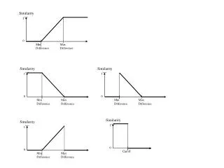
Distance vs. Similarity • Given a feature and its representation associated with each image, we need a metric to compare an image I of the database and the query Q • A distance(d) is defined as follows : d : A x A + A : the set of images : the set of positive real numbers
Distance vs. Similarity • The geometry model - d must satisfy the following properties for all the images I, J and K in A P1 : d(I, I) = d(J, J) self-similarity P2 : d(I, J) d(I, I) minimality symmetry P3 : d(I, J) = d(J, I) P4 : d(I, K) + d(K, J) d(I, J) triangular inequality
Distance vs. Similarity • Tversky(1977) refuted the geometry model - the properties P1 to P3 are not validated by human perception - Symmetry : We are searching a DB using particular query Q so we can not assume the symmetry as obvious - For example (triangle inequality)
Distance vs. Similarity • Tversky proposed non-metric model, Contrast model - An image is characterized as a set of binary features S(A,B) = θ f(A ∩ B) - α f(A-B) - β f(B-A) • However, it is not applied texture or color comparison except shape comparison
From Features to Similarity • The similarity measurements are based on comparison between images features which thus have to be previously extracted - Gray levels - Color with histograms or moments - Texture with the coefficients in the Fourier - Shape for special geometric feature - Structure
Complete vs. Partial Feature • One can take the overall distribution of a given feature in the input image or video as an index • Carson et al. proposed to first segment the image as a set of regions http://dlp.cs.berkeley.edu/photos/blobworld/ - This approach is complex because it requires segmentation step
Complete vs. Partial Feature • Based on key points - Two signals are similar if they have particular feature values spatially located in a consistent order Interest points or key points http://rfv.insa-lyon.fr/~jolion/Cours/ptint.html
Global vs. Local Feature • Global feature value - Take into account all the pixels in the image It is very difficult to summarize to deal with image • Local feature value - A value is computed based on a subset of the image
Global vs. Individual Comparison of Features • There are many different nature of features • It makes it difficult to build a global distance or similarity measure because the indexes have been computed may induce different behavior • The overall similarity is based on a combination of individual similarities • User have to give some weights for the overall similarity computation in some classic systems but, user can’t • The system have to interaction with user to approach the answer
Multidimensional Voting • Voting algorithm(Schmid and Mohr) - Each vector I, of the query image is compared to all vectors J in the DB, which are linked to their images M - If the distance between I, J is below a threshold t, then the respective image M gets a vote - The images having maximum votes are returned to the user • The problem is the threshold strategy is sensitive to the choice of threshold t
Multidimensional Voting • Change the voting algorithm (Wolf) - The means to qualify two points as being a pair is the minimum distance in feature space - To do this, they build a matrix which stores the distance of all possible feature pairs, the row i denoting the key points of the query image, the column j the key points of the compared image • Then, we search the minimum element of the matrix
Multidimensional Voting • This figure shows two examples images and their maps of interest points superimposed in a single image • Corresponding interest points are connected with a straight line
Graph-Based Matching • The information which is a set of points, and each associated with a feature can be abstracted as an attributed relational graph - The vertices of which are the points - The vertices attributes are the vector values - The edges can be established by computing the n-nearest neighbor graph This method is used for image retrieval based on line patterns