Regression Techniques for Performance Parameter Estimation
Regression Techniques for Performance Parameter Estimation. Murray Woodside Carleton University Ottawa, Canada A tutorial for the WOSP/SIPEW Software Performance Workshop, San Jose, Jan 28 2010. Data and Models. delay. delay. x. Trial t: Data Model Predictions

Regression Techniques for Performance Parameter Estimation
E N D
Presentation Transcript
Regression Techniques for Performance Parameter Estimation Murray Woodside Carleton University Ottawa, Canada A tutorial for the WOSP/SIPEW Software Performance Workshop, San Jose, Jan 28 2010
Data and Models delay delay x Trial t: Data Model Predictions configuration parameters ut Calculate yt = h(x, ut) • record or database size matching z • host memory, cores h is the performance model measurement vector ztx are unknown parameters • host utilization, in the performance model • transaction delay Determine x to calibrate h varying configuration parameters x x x x x x x x x x x x x x x x x x x x x x x x x x x x x x x x x x x x disk utilization disk utilization
What is this in aid of? • Performance engineering is in trouble... • time and effort, capability to predict over configurations • Models can help in interpreting data • compact summary • extrapolation (based on performance semantics of h) • configuration, re-architect, re-design • Models created from system understanding need to be calibrated from data • An integrated methodology is possible • paper “Future of Software Performance Engineering”, ICSE 2008
tracing • profiling • instrumenting • testing • load testing • comparing Fact: model and measurement experts do not interact much We have two solitudes, each in its own bubble Performance Measurement Performance Modeling • scenario analysis • high-level models • model generation • sensitivity • scalability • exploration of options
Vision of the “Future of SPE” paper (ICSE 2007):Convergence of Model and Data concerns(this map focuses on performance in design) Test and Measurement Software Performance Model Other uses Perf. Model Solvers Performance Test Design • Specification tools • requirements • design (e.g. UML) • transformation • assembly Perf. Model Builder tools Performance Test Environment Estimation Optimization tools Perf. Model Assembler tools MDD Transformation and Component Assembly tools Knowledge Base Data Repository Platform and Component Specification Library Perf. Submodel Library Other uses Visualization and Diagnosis tools
Solvers Model Generators Load Generators Test Designs Experiment Managers Instrumentation Diagnostic tools (Rule-based Reasoning) Data, databases Statistical Analysis Bridging Models and Data Models Data Model Parameter Estimation • Model Exploitation • problem diagnoses • performance test plans ...towards integrated performance engineering
Starting Point • What kind of measurements? • Where do models come from? • measurements here are averages over a test period • multiple variables are averaged over the same period • models can come from • a basic recipe (e.g., a set of queue servers) • the system configuration • software analysis (e.g. UML annotated by MARTE) • modeling expertise is pretty important... • simplest is best • curve-fit models (not performance models) will be discussed later
Layered queueing model of software services: call-return ...software resources and blocking Queueingmodel of processors ... classes of service ...tokens flow around User or Load Generator App1-CPU App1 App1 App2-CPU C2 C1 App2-CPU Buffer App2 C2 C1 App2 U DB-CPU Q Store Store W W R R Buffer C2 C1 DB U Q App2-CPU Store Database Petri Net Model Resource Operation DB-CPU Execution Flow Different kinds of performance models System...
Example....Automation of performance modeling from annotated UML PUMA Cycle • annotate the UML spec (new standard profile MARTE), • generate the Performance Model • many examples • e.g. PUMA (Perf. by Unified Model Analysis) (paper in WOSP 2005)
User App1 Buf App2 Store DB PModel structure params <<PAstep>>{hostDemand = (2.5,”ms”}> getbuffer <<PAacqResource>>{resource=Buffer, resunits = 1} T Capacity Experiment T = Response time releaseBuffer UML annotated with MARTE profile Users Create a Model from an annotated UML Sequence Diagram tools (e.g. PUMA tools)
View of the Performance Model h(x,u) • h can be any performance model • queueing, layered queueing, petri net, etc • special challenge for simulation models (later) • x contains the unknown parameter values • u contains known parameters that vary from test to test • e.g. the number of users, or the arrival rate • assumption that x does not depend on u (discuss later) • Sensitivity matrix H(x; ut) = h(x; ut)/ x is important • Hij(x; ut) = hi(x; ut)/ xj h u
z N System N jobs throughput f/sec 0:Users demand D1, residence time T1 1: Webserver 3: CGI 2: Disk demand D2 residence T2 demand D3, residence T3 Queuing model example • measurements z • z(1) = delay in webserver • z(2) = delay in disk • z(3) = mean delay in CGI application • a closed system (fixed population) • including “thinking” • an open system has a fixed flow rate, variable population • u = N • with default value 4, • x = [x(1), x(2), x(3)] = [D1, D2, D3]. • simulated data for x = [2, 3, 4] s/response • y = [T1, T2, T3, f]
N jobs, think time Z throughput f/sec demand D1, residence time T1 demand D3, residence T3 demand D2 residence T2 Queueing model • servers represent parts of the system that cause delay (hardware and software) • Users have a latency between getting a response and making the next request (“think time”) • Webserver is the node (processor or collection of processors) (one server or multiserver) running the web server • App is the application processor node • Disk is the storage subsystem
N jobs throughput f/sec demand D1, residence time T1 demand D3, residence T3 demand D2 residence T2 Queueing model (2) A possible situation: • known parameters u = N (number of users), Z • unknown parameters x = [x(1), x(2), x(3)] = [D1, D2, D3]. • “service demands” at nodes in seconds per response • includes multiple visits to a server during a response • measured response delays and throughput z = [T1, T2, T3, f] • Ti = total response delay at node i, summed over a response, sec • f = throughput (flow rate) transactions/sec
Regression: fit and error • measurement = steady-state value + meas’t error • (measurement error comes from averaging over a finite test duration = sampling error) • sampling error is approx normally distributed • variance ~ 1/S, for sample size S • for test number “t” (t = 1, 2, ....) zt = h(x,ut) + approximation error + measurement error • regression assumes the sum of the two errors is normal • zt = h(x,ut) + vt • v is assumed to have constant covariance over t
Regression formulation • minx E(x) E(x) = St (yt − zt)2 (scalar y= h(x,u) and z) E(x) = St (yt − zt)TR-1(yt − zt) (vector y = h(x,u) and z) • Diagonal weight matrix R reflects the relative variances for different measurements in z • called “generalized” least squares • z = h(x,u) + v • Rjj ~ variance of vj
We will need a linearization of h( ) • Regression needs a linear relationship • The sensitivity matrix H =h(x,u)/x is central h1/x1h1/x2 ... ...h1/xn H(x, u) = h2/x1h2/x2 ..... hm/x1hm/x2 ..... • for x near a point x*, h(x,u) = h(x*,u) + H(x*,u)(x – x*) + higher terms (Taylor series)
Gradient solution to Min E An example of an ad hoc numerical minimization approach • E(x) = St (yt − zt)TR-1(yt − zt) = SteTR-1e et = (yt − zt) Iterative solution from some starting x • The gradient vector of E is E(x)/ x = −2 StHT(x; ut) R-1 et • gradient step is: new x = old x - (step parameter)* E(x)/ x
Approximate Newton Raphson iteration • A second-order approximation to E(x) is E(x* + Dx) = E(x*) + ExDx + ½ DxTExxDx + higher terms • A Newton-Raphson step to minimize E is new x = x* + Dx = x* - Exx-1Ex where Ex = E(x)/ x = −2 StHT(x; ut) R-1 et, Exx = 2E(x)/x2 = −2 StHT(x; ut)/xR-1e +2 StH(x; ut)TR-1H(x; ut) ≈ 2 StH(x; ut)TR-1 H(x; ut) (the first term is hard to compute and is small as e → 0)
Approximate Newton-Raphson (2) This can also be seen as successive linear regressions: • At the current estimate x, find the best increment Dx by fitting the Taylor expansion to h for each t, using H: • zt = h(x; ut) + H(x; ut)(Dx) + higher terms + vt • formulate the linear regression problem to find Dx, minDx E(x + Dx) = St (h(x + Dx, ut) − zt)TR-1(h(x + Dx, ut) − zt) • solve as before, but with Dx taking the role of x andH(x, ut) taking the role of B: • Dx = (StH(x, ut)TR-1H(x, ut))-1 (StH(x, ut)TR-1zt) • replace x by x + Dx, repeat to convergence
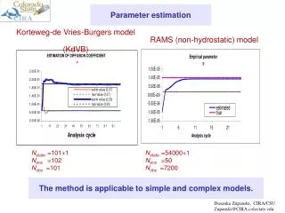
How well does it work?Results for different amounts of data tightest CI (5%)
How to find confidence intervals • Standard regression methods are used to produce confidence intervals (CI) for x • based on each iteration being a linear regression for Dx • the CI is for Dx at convergence • Actually first a covariance matrix P for Dx is calculated: P = (mse) (St HtTR-1Ht)-1 • where mse is an estimator for goodness of fit, given by mse = (St etTR-1et )/(mT n) • m = dimension of y and z • T = number of time points for data • n = dimension of x • mT – n is the number of degrees of freedom • (data – parameters)
Confidence intervals: correlation The Dx are in general correlated, as given by off-diagonal elements of P, so their confidence intervals are not independent • under the assumptions of linearity and normally distributed errors of measurement, Dx are also normal • in 2 dimensions the confidence region is an ellipse, • bounded by a contour of the distribution of Dx point estimate of (x1, x2) x 95% of probability Our CI’s are based on the marginal distributions
Confidence intervals: Math • For simplicity we can base independent CIs on the marginal variances found for each Dxi • estimated variance is Pii • this will be conservative • CI for xi at confidence level a is then xi t(1-a/2; mT-n) (sqrt(Pii )) • where t(1-a/2; mT-n) is a tabulated t-statistic • for a = 0.95 and large mT-n, t( ) → 1.96
Confidence intervals: example • In the example, for 1000-sec trials, the CIs are about 12%, 8% and 5%. Why are they different? • consider case B5: • Best accuracy at the bottleneck, which dominates R
Prediction accuracy can itself be predicted... Case B5, estimated x = 1.850.22, 2.80 0.24, 3.98 0.19 12% 8% 5% Predicted response time vs N data range extrapolated • data points in red x • 10% error band in parameters • 5% error band in predictions (secret is that bottleneck demand parameter is more accurate)
Prediction accuracy calculation 1. near the estimate x cov(Dx) = P 2. also Dy = H(x, u)Dx 3. so C = Cov(y) = Cov(Dy) (since covariance is around the mean) = H(x, u) PHT(x, u) 4. standard deviation for Dyi is sqrt(Cii), so CI for yi is: yi t(1-a/2; mT-n) (sqrt(Cii ))
Another example:the same system with two classes... • The same three queues were simulated with two classes of users • Fitted the same parameters for each class (Dic): • D11, D21, D31 for class 1 • D12, D22, D32 for class 2 • Fitted to measured data • 3 x 10⁶ seconds per experiment • N1 = 1 4 7 10 13 16 19 • N2 = 1 5 9 13 17 21 25 29 • measured the node delays Tic and the class throughputs fc throughput fc/sec • For class c: • throughput fc • At queue i: • demand Dic • total delay Tic • mean customers nic • server utilization Uic
throughput f/sec Results with two classes... • Results were similar This was for 56 data points, each based on 30 blocks of 100000 sec D11 D21 D31 Z1 D12 D22 D32 Z2 Sim: 2 3 4 10 5 10 1 30 Fit: 2.000 3.018 4.033 5.001 9.968 1.026 CI95: .008 .003 .003 .012 .009 .003 .5% .1% .1% .2% .1% .3% • For class c: • throughput fc • At queue i: • demand Dic • total delay Tic • mean customers nic • server utilization Uic
With less data points • 56 long trials is a lot of data... consider using fewer trials: • (1) 13 trials (take every nth row of data)(mT – n = 104 – 6 = 98 df) parameter D11 D21 D31 D12 D22 D32 estimate 1.998 3.014 4.010 5.007 9.975 1.025 95% conf int 0.015 0.006 0.005 0.024 0.017 0.006 • percent confidence intervals are doubled compared to 56 points... • With even less data, accuracy is still OK: (2) 7 runs: D11 D21 D31 D12 D22 D32 mT-n = 56-6 = 50 est 2.002 3.017 3.999 5.012 9.947 1.021 CI 0.023 0.009 0.012 0.035 0.023 0.012 50% more than (1) (3) 3 runs: D11 D21 D31 D12 D22 D32 mT-n = 24 – 6 =18 est 2.004 3.016 4.000 4.969 9.957 1.027 CI 0.039 0.014 0.017 0.069 0.044 0.018 more than double (1)
Suppose we have different measurements in the data points • Class response times Rc and device utilizations Uic are relatively easy to measure • with data on R only, the order of queues is lost (there is no queue-specific data)
Observations on fitting queuing models 1. Always fit a constant (a think time) to a delay measurement • a latency term in the delay • it stands for system elements missing in the model 2. Many systems have a dominant bottleneck resource • they behave rather like a single queue plus a latency • The latency stands for delays at all the other resources • to obtain good estimates for the other resources • include data in the non-bottleneck region • include data about those resources (e.g., their utilization)
Observations (2) 3. Other queuing models can be used • more queues, or fewer • each model produces a goodness of fit E • you can test the models for significance (a significant reduction in E) • “did the extra parameter produce enough reduction” • you can also examine the confidence intervals • models with too much detail tend to give large intervals on some or all parameters • the parameters can substitute for each other
Significance testing for model structure • To tell if you have the right model structure • call the model m1, its number of fitted parameters n1, and its goodness of fit, E1 = SteTR-1e • another model m2 with n2 parameters has fit E2 • is m1 significantly better than m2? • this requires an F-test: • m1 is better than m2 at level a if: • F-statistic > critical F-value (tabulated) at level a • for 95% probability it is better, a = 0.05 [(E2−E1)/(n1−n2)]/[E2/(mT−n2−1)] > F(n2−n1, mT−n −1, a)
Significance vs a simpler 2-queue model, on data for 3 queues • m1 has three queues with E1 = 32.9, n1 = 6, m = 8, T = 56 D11 D12 D13 D21 D22 D23 Sim: 2 3 4 5 10 1 Fit: 2.000 3.018 4.033 5.001 9.968 1.026 CI95: .008 .003 .003 .012 .009 .003 • m2 has two queues with E2 = 4034, n2 = 4, m = 6, T = 56 D11 D12 D21 D22 Fit: 2.13 3.24 4.88 9.68 ..for class 2 it has “chosen” queue 1,2 CI95: .087 .038 .144 .107 .. about 10 times as big • F = [(E2−E1)/(n2−n1)]/[E2/(mT−n2−1)] = [(4034−33)/(6−4)]/[4034/(448−6−1)] = 220.4 • tabulated F(2, 441, .05) = 19.5 .... so, m1 is better.
Observations (3) • In open queueing systems it is well known that the variance of a measure increases with load • Mean delay ~ 1/(1-U) • Variance ~ 1/(1-U)2 for many disciplines • in the three-queue system the variances of T11 and T22 are: 4. Measurement error is not constant over trials So, rather a lot of variation. However the coefficient of variation is rather stable...
Dealing with varying measurement errors • The weight matrix W = R-1 can be a function of the sample t, provided it is known. Then • min E(x) = St (yt − zt)TWt(yt − zt) • only ad hoc approaches are available, • i.e. if we think the coefficient of variation is constant, we could set Wii,t equal to (constanti) x zit2 • but ignoring the variation does not seem to work too badly...
Observations (4) 5. Is the violation of regression assumptions a serious issue for good fitting? • It seems not. The key assumptions are • linear h in x • normal measurement errors with const variance • if these are true, the residuals have a multivariate normal distribution, and the fitted parameters also • shown by elliptical contours of the probability density function • and elliptical contours of E(x) centered around the fitted value of x
Contours of E for a two-Class Model • If the regression approximation assumptions are satisfied • (linear h, normal error) • then E(x) is normal with estimated mean Xest, covariance matrix P. • a 2-dimensional normal distribution has elliptical contours • Here we see that contours of E are nearly elliptical, so the assumptions are supported. D2 from 2.5 to 3.5 in steps of 0.025 D1 from 9.5 to 10.5 in steps of 0.05
Confidence region for D1, D2 • The true confidence region for any % is the inside of one of these contours • The separate CI’s we calculate are for the marginals of E... shaped like the box (ours are actually very small) D2 from 2.5 to 3.5 in steps of 0.025 D1 from 9.5 to 10.5 in steps of 0.05
Now consider more structured and complex models • Real systems have more structure to their resources, than a simple queueing model • this may or may not be important • Extended queueing models can capture this extra structure • memory resources • process resources • etc. • Layered queues are a canonical form for extended queueing, • adapted to layered service systems • also usable on other systems, eg event-based systems
users Users UserP [think=5] {$nuse rs=1:50} {inf} (1) webServ WSP WebServer [$wsD=0.4] {2 } {$wsThreads=3} (0.7) appOp Application AppP [$apDph1=0.2, {$mApp=1} {1 } $apDph2=0.2]] (0.1) (1.5,0.7) dirServ Directory dbOp DataBase [$dirD=0.1] {1} [$dbD=0.1] {1} UserP {1 } Layered system example Entry Task u = $nusers Example: basic tiered service system Extended queueing model • Reflects the interaction architecture • Tasks with {multiplicity} • Entries (operations) with [cpu demand] • Calls with (frequency) • Hosts, with {multiplicity} Call Host
users Users UserP [think=5] {$nuse rs=1:50} {inf} (1) webServ WSP WebServer [$wsD=0.4] {2 } {$wsThreads=3} (0.7) appOp Application AppP [$apDph1=0.2, {$mApp=1} {1 } $apDph2=0.2] (0.1) (1.5,0.7) dirServ Directory dbOp DataBase [$dirD=0.1] {1} [$dbD=0.1] {1} UserP {1 } Layered system example u = $nusers • In this model, variables like $wsD= 0.4 show the true (simulation) value, • 7 parameters (in red) were estimated • CPU demands of operations, • thread pool size (multiplicities) of servers • integer parameters for the multiplicities • asynchronous operation in “second phase” of the application • $nusers was controlled x = $dirD $wsD $appDph1 $appDph2 $dbD $mApp $wsThreads
Estimation results Parameter • Low sensitivity => low accuracy • Integer parameters were successfully estimated Accuracy low OK OK low high OK? OK
Fitted Curve: Prediction accuracy (response time) • Good accuracy because the sensitive parameters were accurately estimated Think time = 5 sec, as for estimation = 15 sec
How to do it • I have a bunch of data, how do I fit models? • first, I need a hypothesis for a model • a think time and a set of queues will do • if it is test data with a load driver, a closed model is indicated • if it is data recorded “in the wild” with a varying load, try a closed approximation (fix a large N, and for each test set Zt = N/ft) • with multiple measures averaged over each run, the relative variance of each must be estimated for R • roughly. The simplest assumption is equal variances • set initial values and iterate. I use MATLAB... • The model calculation h(x) is done by a function • The sensitivity matrix H is computed by finite differences • For integer-valued parameters, use a difference = 1, and round the regression results after each iteration
Dealing with problems • Don’t Panic if a model seems to be nonsense • look at its predictions • there may be a trend, like underestimating delay at high loads, that indicates additional resource use (e.g. paging) • you may have to constrain the model more, or add more freedom to fit • include a latency, it vacuums up simple things that have been left out • some models have undetermined parameters. For instance a pair of parameters may have interchangeable effects on the measured variables • so that many combinations of values can be fitted, with the same E... fix one, or simplify the structure
Rank of H • the iteration may stop on a singular matrix M = StH(x, ut)TR-1H(x, ut) • examine the rank of M • it must be at least n • h must be sensitive to every parameter x, in some condition u. • a high condition number of M may signal poor convergence behaviour • you may have to introduce more variation in ut • more variation in the test conditions • this amounts to design of better tests, for predictive purposes
Open systems • For modeling purposes I personally prefer to model open systems as if closed • better behaved calculations, you never get infinite response times or infeasible processor demands • choose a very large N for the population • to get roughly a fixed throughput f/sec, calculate Z = N/f • if I want to extrapolate to higher throughputs I need a big enough N
Where do curve-fit models come in? • e.g., a polynomial curve fitted to each measure • you can do this with the same techniques • hi (x, u) = polynomial in elements of u, with coefficients x to be found. • such a model can be compared by an F test • the disadvantage of ad hoc functions for h is the lack of performance semantics • extrapolation is less robust