Insights on Transformation Invariance in Parameter Estimation
Explore the impact of transformations on various algorithms such as DLT, and learn about the importance of normalization in improving accuracy. Discover robust estimation methods like RANSAC for outlier detection. Dive into automatic computation of homography for image analysis.


Insights on Transformation Invariance in Parameter Estimation
E N D
Presentation Transcript
Invariance to transforms ? will result change? for which algorithms? for which transformations?
Non-invariance of DLT Given and H computed by DLT, and Does the DLT algorithm applied to yield ? Answer is too hard for general T and T’ But for similarity transform we can state NO Conclusion: DLT is NOT invariant to Similarity But can show that Geometric Error is Invariant to Similarity
Normalizing transformations • Since DLT is not invariant, what is a good choice of coordinates? e.g. • Translate centroid to origin • Scale to a average distance to the origin • Independently on both images
Importance of normalization 1 ~104 ~102 ~102 ~102 ~102 ~102 1 ~104 orders of magnitude difference! Without normalization with normalization Assumes H is identity; adds 0.1 Gaussian noise to each point. Then computes H:
Normalized DLT algorithm • Objective • Given n≥4 2D to 2D point correspondences {xi↔xi’}, determine the 2D homography matrix H such that xi’=Hxi • Algorithm • Normalize points • Apply DLT algorithm to • Denormalize solution
Iterative minimization metods Required to minimize geometric error • Often slower than DLT • Require initialization • No guaranteed convergence, local minima • Stopping criterion required
Initialization • Typically, use linear solution • If outliers, use robust algorithm • Alternative, sample parameter space
Iterative methods Many algorithms exist • Newton’s method • Levenberg-Marquardt • Powell’s method • Simplex method
Robust estimation • What if set of matches contains gross outliers? ransac least squares Filled black circles inliers Empty circles outliers
RANSAC • Objective • Robust fit of model to data set S which contains outliers • Algorithm • Randomly select a sample of s data points from S and instantiate the model from this subset. • Determine the set of data points Si which are within a distance threshold t of the model. The set Si is the consensus set of samples and defines the inliers of S. • If the subset of Si is greater than some threshold T, re-estimate the model using all the points in Si and terminate • If the size of Si is less than T, select a new subset and repeat the above. • After N trials the largest consensus set Si is selected, and the model is re-estimated using all the points in the subset Si
Distance threshold Choose t so probability for inlier is α (e.g. 0.95) • Often empirically • Zero-mean Gaussian noise σ then follows distribution with m=codimension of model (dimension+codimension=dimension space)
How many samples? Choose N so that, with probability p, at least one random sample of s points is free from outliers. e.g. p=0.99; e =proportion of outliers in the entire data set
Acceptable consensus set? • Typically, terminate when inlier ratio reaches expected ratio of inliers; n = size of data set; e = expected percentage of outliers
Adaptively determining the number of samples e is often unknown a priori, so pick worst case, e.g. 50%, and adapt if more inliers are found, e.g. 80% would yield e=0.2 • N=∞, sample_count =0 • While N >sample_count repeat • Choose a sample and count the number of inliers • Set e=1-(number of inliers)/(total number of points) • Recompute N from e • Increment the sample_count by 1 • Terminate
Automatic computation of H • Objective • Compute homography between two images • Algorithm • Interest points: Compute interest points in each image • Putative correspondences: Compute a set of interest point matches based on some similarity measure • RANSAC robust estimation: Repeat for N samples • (a) Select 4 correspondences and compute H • (b) Calculate the distance d for each putative match • (c) Compute the number of inliers consistent with H (d<t) • Choose H with most inliers • Optimal estimation: re-estimate H from all inliers by minimizing ML cost function with Levenberg-Marquardt • Guided matching: Determine more matches using prediction by computed H • Optionally iterate last two steps until convergence
Example: robust computation Interest points (500/image) Left: Putative correspondences (268) Right: Outliers (117) Left: Inliers (151) after Ransac Right: Final inliers (262) After MLE and guided matching