Download
1 / 9
90 likes | 125 Views
Explore inverse kinematics problems, discover analytic solutions and learn about the Jacobian matrix. Dive into numeric solutions and different cases of solving inverse kinematics. Understand overconstrained, underconstrained, and single solution systems, with examples and methods like Cyclic Coordinate Descent.

E N D
CSCI480/582 Lecture 13 Chap.3.2 Inverse Kinematics Feb, 20, 2009
Outline • Inverse Kinematics Problem • Analytic Solutions to Inverse Kinematics • The Jacobian Matrix • Numeric Solutions to Inverse Kinematics • Case 1: Direct Jacobian Inversion • Case 2: Pseudo-inversion of Jacobian • Case 3: Adding controls to the solver • Cyclic Coordinate Descent method
Inverse Kinematics Problems • Given the desired position and/or oriention of the end effector (pose vector), calculate the joint values required to attain that configuration. • Overconstrained system: the desired position and/or orientation is outside the reachable workspace • Underconstrained system: multiple joint values can attain the same configuration • Single solution system • Given initial and final pose vectors, the animation can be generated by interpolating the joint values calculated from the two poses.
(x, y) L2 ө2 L1 ө1 Analytical solution for simple systems Example: A two-link arm in 2-D space with two rotational DOF. The first arm is anchored at the origin with a length of L1, and second arm has a length of L2.
The Jacobian Matrix • Representing the 1st-order partial derivatives of a function with multiple input variables and multiple output variables. • For articulation movement, often the expected end motion dP is defined by the user, the system needs to move the model using the joint transformation matrices dθ to approach that requested end effector motion.
Numeric Solutions to Inverse Kinematics – Case 1 with Invertible Jacobian Matrix • When J is determinant is non-zero, given the end effector velocities, the joint parameter velocities can be calculated as
Numeric Solutions to Inverse Kinematics – Case 2 Pseudo-inverse Jacobian • Especially useful for ill-posed systems • When J is not invertible • The solution is optimum in generating the closest approximation to the target end-effector velocity in terms of the sum of the squares of the differences between result and target.
Numeric Solutions to Inverse Kinematics – Case 3 Adding controls • More specific constraints on the joint parameters z(θ) can be added to the linear solver without affecting the estimation result
Cyclic Coordinate Descent • Solving joint parameters in a sequential order Useful Numeric solver library • GNU Scientific Library • http://www.gnu.org/software/gsl/