Phase V Watershed Model
Phase V Watershed Model. We have 1994-2000 flows, revised March 2006. Used to drive CH3D We have May 2006 Phase V loads for WQM. Revisions to Phase V loads are possible. Phase IV.3 Loads. Phase V Loads. Phase IV.3 Loads. Phase V Loads. Phase IV.3 Loads. Phase V Loads. Phase IV.3 Loads.

Phase V Watershed Model
E N D
Presentation Transcript
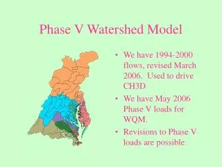
Phase V Watershed Model • We have 1994-2000 flows, revised March 2006. Used to drive CH3D • We have May 2006 Phase V loads for WQM. • Revisions to Phase V loads are possible
Phase IV.3 Loads Phase V Loads
Phase IV.3 Loads Phase V Loads
Phase IV.3 Loads Phase V Loads
Phase IV.3 Loads Phase V Loads
Phase IV.3 Loads Phase V Loads
Conclusions • Total nitrogen and phosphorus loads appear to go down • Tributaries are more sensitive than main bay. Changes largely in most upstream stations • Scatter is reduced for nitrogen and phosphorus • No consistent difference for solids • No fundamental change in calibration status
For every model cell, we have the following area increments: • < 0.5 m • 0.5 m < d < 1 m • 1 m < d < 1.5 m • 1.5 m < d < 2 m Keeping track of these areas and the SAV within will allow us to compute SAV area and compare to CBP data base
Status • We will complete detailed examination of SAV in four key segments, one for each species. • We will look at annual areas for total and ten largest segments • SAV is currently implemented for one species, Vallisneria, everywhere. We need to tune and incorporate two more species
CBP criteria for SAV survival is optical depth less than 1.6 to 2
Optical Model • Model developed by Charles Gallegos, SERC • Rigorous calculation of diffuse light attenuation based on inherent optical properties of color, total suspended solids, chlorophyll • Parameter set from this study and other CBP-sponsored efforts
Optical Model • Parameter set varies seasonally and, potentially, in 78 CBPS • A good deal of judgment was involved in parameter assignment when observations were unavailable. • The calculation is enormously time-consuming. Chuck created a 2,000,000 element look-up table that is incorporated in our model.
Old Attenuation Model New Attenuation Model
Old Attenuation Model New Attenuation Model
Old Attenuation Model New Attenuation Model
Estuarine Phosphorus Model • Initial coding of PIP in water quality model • PIP assumed to be completely inert • Behaves as TSS
70% of Choptank PP is PIP 47% of Potomac PP is PIP
58% of Susquehanna PP is PIP 62% of Patuxent PP is PIP
No PIP With PIP
No PIP With PIP